OEIS A160136

A sequence by Philippe Deléham, this page written by Michael Thomas De Vlieger, St. Louis, Missouri, 2020 1001, with collaboration from David J. Sycamore of Mevagissey, England, UK.

Abstract.

We examine the “lodumo” transform of the Fibonacci sequence mod m noted herein as lod_m F(n), linking it with a function g(x) associated with base-(m + 1) digital roots. A third method of generating the sequence is given related to observations of the plot of lod_m F(n), which exhibits a repetitive pattern that obeys the Pisano period π(m). Specifically, we note a method to extract the slopes m f_s / π(m) of quasi-linear constellations of points in the plot, where f_s is a slope factor, the provenance of which remains unknown. We offer several algorithms to plot and analyze the sequences, and through a complete automation of all the processes that we have employed for lod₉ F(n), we attempt to resolve some of the reasons behind residues mod π(m) and mod m that give rise to certain line constellations in the plot.

Introduction.

Philippe Deléham devised a sequence transform he entitled “lodumo” (a reversal of the syllables of “modulo”) and abbreviated lod_m s, where s(n) is the sequence to transform, and defined as the least number not in a(n) such that a(n) ≡ s(n) (mod m). [1]

The resultant sequence a(n) contains no duplicated terms and is equivalent to s(n) mod m.

Furthermore, a(n) is a permutation of the nonnegative integers if and only if all residue classes mod m appear infinitely often in s(n) mod m. We know this is the case for m = 9 and s being the Fibonacci sequence, as 9 occurs in A079002, the list of m such that F(n) mod m forms a complete residue system. It is not always the case that lod_m of the Fibonacci sequence is a permutation of the natural numbers, but often is for small m.

The Fibonacci sequence, here defined as F(n) = OEIS A45(n), begins

0, 1, 1, 2, 3, 5, 8, 13, 21, 34, 55, 89, 144, …

This is a linear recurrence with signature (1, 1) beginning from index 0 with {0, 1}. Essentially, we sum the penultimate and last terms F(n − 2) and F(n − 1) to obtain F(n).

It is known that F(n) mod m is periodic according to the Pisano number π(n) = A1175(n). We might observe this decimally in the periodicity of the final digit of the Fibonacci numbers as n increases, though unfortunately π(n) sets a record at n = 10, with π(10) = 60.

We observe that π(9) = 24. Therefore, we see that A7887(n) = F(n) mod 9 has period 24:

0, 1, 1, 2, 3, 5, 8, 4, 3, 7, 1, 8, 0, 8, 8, 7, 6, 4, 1, 5, 6, 2, 8, 1,
0, 1, 1, 2, 3, 5, 8, 4, 3, 7, 1, 8, 0, 8, 8, 7, 6, 4, 1, 5, 6, 2, 8, 1,
0, 1, 1, 2, 3, 5, 8, 4, 3, 7, 1, 8, 0, 8, 8, 7, 6, 4, 1, 5, 6, 2, 8, 1,
...

We might generate A7887(n) by taking the terms F(n) mod 9, or simply constraining the sum A7887(n − 2) + A7887(n − 1) mod 9. Therefore, the sequence might arise without engaging large numbers and occur only among the residues (mod 9). We note that all the residues (mod 9) are present among the 24 repeated terms.

Consider a(n) = A160136(n) = lod₉ F(n). Deléham arrives at this sequence conventionally per definition via the self-referential function f(n) (see Code 1):

If (a(n − 2) + a(n − 1) ) mod 9 + 9j ∈ a(n)
then increment j until FALSE,
else append (a(n − 2) + a(n − 1) ) mod 9 + 9j to a(n).

Retaining the index offset n ≥ 0 from A45, a(n) starts:

0, 1, 10, 2, 3, 5, 8, 4, 12, 7, 19, 17, 9, 26, 35, 16, 6, 13, 28, 14, 15, 11, 44, 37, ...

By definition these numbers have the residues (mod 9):

0, 1, 1, 2, 3, 5, 8, 4, 3, 7, 1, 8, 0, 8, 8, 7, 6, 4, 1, 5, 6, 2, 8, 1, ...

and are only increased by some multiple 9j so as to present a number unique to a(n). Therefore, A7887(n) is simultaneously F(n) mod 9 and A160136(n) mod 9.

Sycamore’s construction of a(n).

Sycamore arrives at a(n) via another method relating to decimal digital roots d(n) = A010888(n). Let d(n) be the fixed point of recursively adding the decimal digits of | n |. Thus, d(999) = 9 + 9 + 9 = 27 → 2 + 7 = 9. We note that the decimal digital root is always a single-decimal-digit number, but may only be 0 when n = 0, and we are left with a nonzero decimal digit in the case of n ≠ 0. Regarding the digital root funcion d(n):

d(0) = 0;
d(n) = ((n − 1) mod 9) + 1

and further, that n mod 9 merely renders d(n) = 9 instead as 0.

Sycamore defines b(n) as:

b(0) = 0, b(1) = 1, then,
b(n+1) is smallest number not yet seen in b(n) such that d(b(n+1)) = d(b(n−1) + b(n)).

We consider sequence b(n), based on a self-referential function g(n), with g(0) = 0, g(1) = 1 and the function g(n) (See Code 2):

If d(g(n − 2) + g(n − 1) ) + 9j ∈ b(n)
then increment j until FALSE,
else append d(g(n − 2) + g(n − 1) ) mod 9 + j to b(n).

b(2) = 10, since 0 + 1 = 1, but b(1) = 1. We see that (1 + 9) mod 9 is congruent to 1 mod 9, and further that 10 is not in b(n).
b(3) = 2 since 1 + 10 = 11 → 1 + 1 = 2, etc., so as to arrive at the sequence b(n):

0, 1, 10, 2, 3, 5, 8, 4, 12, 7, 19, 17, 9, 26, 35, 16, 6, 13, 28, 14, 15, 11, 44, 37, ...

and it is clear that a(n) = b(n).

Analysis of the plot of a(n).

Figure 3.1 shows a seemingly unremarkable plot of a(n) for 0 ≤ n ≤ 1000:

The plot exhibits two classes of terms. In red, we see terms in a “upper” quasilinear arrangement, and in blue, terms in a “lower” quasilinear arrangement. For the sake of simplicity in this work we refer to these as “red” or “blue” terms in an upper or lower line respectively. We say “quasilinear” for the reason that indeed the points do not define a line but dither around it, and indeed, the red line represents a great jump from a blue term at times, from which eventually the function returns to blue.

Figure 3.2 shows only 144 terms, with the red and blue lines dotted in among the plotted terms, and gridlines governed by Pisano period π(9) = 24 and a(n + 24) − a(n) = 45 pertaining to red points (see Code 5):

Here we see that there is repetition in the arrangement of the points about the lines associated with the Pisano period 24. Here we call the set of points that cluster and pertain to a given line, delimited by integer multiples of π(m), a “constellation”.

Figure 3.3 plots a(n) for 0 ≤ n ≤ π(9), writing coordinates (x, y) ← (n, a(n)) (See Code 6):

From this, and recognizing the properties of the lodumo transform, congruences, and the Fibonacci numbers, we find the slopes of the red and blue lines.

For red, we have the displacement a(n + 24) − a(n) = 45, thus the slope m_red = 15/8.

For blue, we have the displacement a(n + 24) − a(n) = 18, thus the slope m_blue = 3/4.

Furthermore, we might group the terms in a(n) into two classes as to their residue r (mod 24). The red terms have n ≡ r (mod 24) for r in {1, 2, 6, 10, 11, 13, 14, 18, 22, 23}, while the blue terms have r in {0, 3, 4, 5, 7, 8, 9, 12, 15, 16, 17, 19, 20, 21}. There are 10 residues in the red constellation, and 14 residues in the blue constellation.

Figure 3.4 plots the red and blue residues on a clock-like arrangement to accentuate the symmetry of these residues r (mod 24):

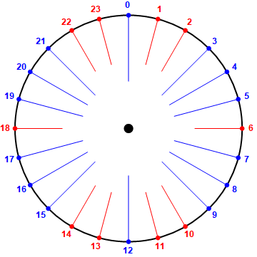
Thus residues r = ±1, ±2, or 6 (mod 12) are in red, and the balance are in blue.

Mapping the red and blue residue classes to A7887(n) for 0 ≤ n ≤ 23, we have:

0, 1, 1, 2, 3, 5, 8, 4, 3, 7, 1, 8, 0, 8, 8, 7, 6, 4, 1, 5, 6, 2, 8, 1

By this it is evident that, if a(n) ≡ ±1 (mod 9), then it occurs in the red line, else it appears in the blue line.

Since we might divide a(n) into two linear arrangements, given the slopes R(n) = 15/8 × n (red) and S(n) = 3/4 × n (blue), we now turn to attempting to generate a(n) not through the self-referential functions f(n) or g(n), but instead through the conditional slopes and the displacements that obey the Pisano period 24. Computationally, this is the fastest method of generating a large number of terms of a(n).

Essentially, we need only use the first 24 terms of a(n), subtracting a(n) − R(n mod 24) for a(n) ≡ ±1 (mod 9) and S(n mod 24) − a(n) otherwise. From this we obtain a finite series of 24 displacements D.

Examples.

For n ≡ 0 (mod 24) we use a(0) = 0, a(24) = 18, a(48) = 36, etc. Since these numbers are congruent to 0 (mod 9), they are blue and we employ S(n) = 3/4 × n, thus 0 − 0 = 0. Thus D(0) = 0.

For n ≡ 1 (mod 24) we use a(1) = 1, a(25) = 46, a(49) = 91, etc. Since these numbers are congruent to 1 (mod 9), they are red and we employ R(n) = 15/8 × n, thus 15/8 − 1 = 7/8. Thus D(1) = 7.

For n ≡ 2 (mod 24) we use a(2) = 10, a(26) = 55, a(50) = 100, etc. Since these numbers are congruent to 1 (mod 9), they are red and we employ R(n) = 15/8 × n, thus 30/8 − 10 = −50/8. Thus D(1) = −50.

For n ≡ 3 (mod 24) we use a(3) = 2, a(27) = 20, a(51) = 38, etc. Since these numbers are congruent to 2 (mod 9), they are blue and we employ S(n) = 3/4 × n, thus 9/4 − 2 = 1/4. Thus D(0) = 2 (recalling that we are multiplying all the displacements by 8, their common denominator, so as to render a series of integers).

Etc.

This yields the following displacements in D(i), indexed 0 ≤ i ≤ 23:

0, −7, 50, −2, 0, 10, −26, −10, 48, 2, 2, −29, 0, 13, 70, 38, −48, 2, −46, −2, 0, −38, 22, −49

Figure 3.5 plots these on the radial plot introduced by Figure 4, with gray concentric circles indicating D/8 in units, with the black circle indicating D/8 = 0, outward circles a positive D/8, and interior circles a negative D/8. The scale of the spacing of the concentric circles is arbitrary so as to make the diagram legible (See Code 7):

A third, efficient construction of a(n).

Using this conditional approach and given the displacements D, we may define a(n) = A160136(n) as follows (see Code 3):

If F(n mod 24) mod 9 ≡ ±1
then 15/8 × n + D(n mod 24),
else 3/4 × n + D(n mod 24).

This method avoids the self-referential assurance checking of f(n) or g(n) and allows us to compute an individual value a(n) for any nonnegative n.

What remains to be determined is a reason for the displacements and the resultant arrangement of the displacements of points along the lines.

The slope factors of lod_m F(n).

We have found the slopes of the quasilinear features in the plot of lod₉ F(n). These are 45/24 and 18/24, the numerators taken from the primitive displacements 45 (for the upper line) and 18 (for the lower line) gleaned from points (x, y) = (n, a(n)), with x offset by π(9) = 24. In attempting to understand these numerators (for the denominator is clearly the Pisano number) we note that these are multiples of 9.

Since we are now attempting to understand the features of these slope factors and having only studied the case m = 9, we turn to other bases m. Indeed, an initial reaction, citing Sycamore’s approach using the self-referential function g(x), would be to study m = 5, as it would then pertain to the senary (i.e., base 6) digital roots. When we adjust the algorithm so as to generate lod₅ F(n), we find, astonishingly, that there is only one line in its plot. We might surmise that it is because 5 is prime, but indeed, looking at other m, we find that 5 somehow has 1 line, but that is relatively rare.

Indeed we might devise a sequence ℓ(m), the number of quasilinear periodic features in the plot of lod_m F(n). In other words, ℓ(m) is the number of constellations for m. In order to achieve this, we might write a program that computes π(m) then generates s(m,n) = lod_m F(n) for 0 ≤ n ≤ 2π(m), finding all the displacements (x, y) for x = {n, n + π(m)}. From this dataset we take the union to arrive at a set of primitive values.

Table 5.1 lists values of ℓ(m) for 2 ≤ m ≤ 50 (Click here for a table of m, ℓ(m) for 2 ≤ m ≤ 1000 in the style of an OEIS b-file):

2, 2, 2, 1, 4, 3, 3, 2, 2, 3, 3, 2, 4, 2, 4, 2, 3, 3, 2, 3, 5, 3, 3, 1, 3, 3, 4, 3, 4, 3, 4, 4, 2, 3, 3, 2, 3, 3, 3, 3, 5, 3, 4, 2, 3, 3, 3, 3, 2, 3, ...

We note the following regarding indices m of particular values of ℓ(m):

ℓ(m) = 1 for m in {5, 25, 125, 625, …}, it seems any nonnegative perfect power of 5, aligning somewhat with A079002.
ℓ(m) = 2 for m in {2, 3, 4, 9, 10, 13, 15, 17, 20, 34, 37, 45, 50, 53, 61, 65, 73, 75, 85, 89, 97, 100, …}.
ℓ(m) = 3 for m in {7, 8, 11, 12, 18, 19, 21, 23, 24, 26, 27, 29, 31, 35, 36, 38, 39, 40, 41, 43, 46, 47, 48, …}.

The first positions of values x in ℓ(m) for 2 ≤ m ≤ 1000 appear in Table 5.2 below:

x    m
------
1    5
2    2
3    7
4    6
5   22
6   66
7  242
8  426
...

Table 5.3 lists the ℓ(m) primitive displacements d_p that, when divided by π(m), yield the ℓ(m) slopes d_p/π(m) of the quasi-lines of the plot of lod_m F(n).

 m   primitive displacements
----------------------------
 2:   2     4;
 3:   6     9;
 4:   4    12;
 5:  20;
 6:  12    18    24    36;
 7:   7    14    28;
 8:   8    16    24;
 9:  18    45;
10:  40    80;
11:  11    22    33;
12:  12    24    60;
13:  26    52;
14:  14    28    56   112;
15:  30    45;
16:  16    32    48    64;
17:  34    68;
18:  18    36    72;
19:  19    38    57;
20:  40   120;
21:  21    42    63;
22:  22    44    66    88   132;
23:  23    46    92;
24:  24    48    72;
25: 100;
26:  52   104   208;
...      

It is clear that these primitive displacements must be multiples f_s × m, thus the slope of any quasi-line in the plot of lod_m F(n) can be expressed as f_s × m/π(m). Therefore we arrive at the slope factors f_s in Table 5.4 below, arranged so as to align particular slope factors in the same columns in numerical order:

 m   slope factors
---------------------------
 2:  1  2
 3:     2  3
 4:  1     3
 5:           4
 6:     2  3  4     6
 7:  1  2     4
 8:  1  2  3
 9:     2        5
10:           4           8
11:  1  2  3
12:  1  2        5
13:     2     4
14:  1  2     4           8
15:     2  3
16:  1  2  3  4
17:     2     4
18:  1  2     4
19:  1  2  3
20:     2           6
21:  1  2  3
22:  1  2  3  4     6
23:  1  2     4
24:  1  2  3
25:           4
26:     2     4           8
...

The range of f_s pertaining to any m resemble a list of divisors of some number, with certain factors effaced. The columns 2 and 4 seem strong, with perhaps a preference for even values.

Figure 5.1 plots the scale factors f_s for 2 ≤ n ≤ 216 as above, with (n, f_s) → (x, y), i.e., rotated counterclockwise:

Figure 5.2 shows 2 ≤ n ≤ 864:

The scale factors indeed seem to prefer even values as f_s increases, with more weight given to smaller values.

The records r for the sequence of the maximum scale factors for m occur at the following indices m:

 r     m
--------
 2     1
 3     2
 4     4
 6     5
 8     9
10    65
11    80
14    97
22   241
23   528
28   685
44   725
...

A study of lod_m F(n) for particular m.

We have written code that automatically analyzes the lodumo-m transform of the Fibonacci sequence. The program finds the Pisano number π(m), calculates all the displacements within lod_m F(n) for 0 ≤ n ≤ 2π(m) to arrive at the list of ℓ(m) slope factors f_s. Given these, it calculates the panel of displacements in D for each n mod π(m). It plots lod_m F(n) in three scales as seen in figures in this work, and generates the symmetry and displacement diagrams also seen above. Because of the possible multiplicity of examinations that can be fostered using this algorithm, we focus on m that may appear to offer interest.

We shall examine m = 2 with ℓ(2) = 2, a complete residue system and thus a permutation of the natural numbers tantamount to OEIS A6369. That sequence is defined as a(3n − 2) = 4n − 3, a(3n − 1) = 4n − 1, a(3n) = 2n. This is perhaps the simplest non-trivial case for lod_m F(n).

We have a single constellation for m = 5, also a complete residue system.

The smallest m with ℓ(m) = 3 is 7, a complete residue system which pertains to octal digital roots per Sycamore’s approach.

The smallest m with ℓ(m) = 4 is 6, a complete residue system.

Finally, we look at m = 22, the least m with ℓ(m) = 5, not a complete residue system, thus not a permutation of the natural numbers.

The color-codes in the algorithms used to generate the plots and diagrams are automatically generated by assuming ℓ(m) = 1 in black (or red), ℓ(m) = 2 in blue and red, but ℓ(m) = k dividing the color-circle evenly into k parts, justifying the highest slope factor to red. Furthermore the algorithm darkens hues between orange and teal, since these tend to be fairly brilliant and get lost, printed on a white background.

For reference we give a chart of residues (mod m) for 2 ≤ m ≤ 26 and their coverage in the appendix.

Case m = 2.

We examine m = 2, thus, a(2, n) = lod₂ F(n), which is tantamount to OEIS A6369. The sequence is thus simple:

With a(0) = 0, a(1) = 1,
a(3n − 2) = 4n − 3,
a(3n − 1) = 4n − 1,
a(3n) = 2n.

Therefore a(2, n) begins:

0, 1, 3, 2, 5, 7, 4, 9, 11, 6, 13, 15, 8, 17, 19, 10, 21, 23, 12, 25, 27, 14, 29, 31, 16, 33, 35, 18, ...

The lodumo-2 transform of the Fibonacci numbers obeys the Pisano number π(2) = 3. The plot features two quasi-lines. Therefore we multiply the slope factors f_s, 1 and 2, by 2/3 to obtain the slopes 2/3 and 4/3 respectively. Simply using the slope factors, we see that there is 1 residue for f_s = 1 and 2 residues pertaining to f_s = 2. Even n have f_s = 1 and odd n have f_s = 2. The displacement list for the residues of lod₂ F(n) mod π(2) is {0, 1, −1}, each with denominator 3.

Figure 6.2.1 is a graph of lod₂ F(n) = A6369.

Case m = 5.

This work concerned itself with m = 9, the plot of which generated ℓ(9) = 2 quasi-lines as for m = 2. We have shown that ℓ(m) varies, and that for 5 and its perfect powers (at least to 625), we have ℓ(m) = 1. All m that are perfect powers of 5 exhibit a complete residue system. Therefore the case a(5, n) would seem to merit evaluation. The sequence begins:

0, 1, 6, 2, 3, 5, 8, 13, 11, 4, 10, 9, 14, 18, 7, 15, 12, 17, 19, 16, 20, 21, 26, 22, 23, 25, 28, 33, ...

The sequence a(5, n) = lod₅ F(n) obeys the Pisano number π(5) = 20. The plot of a(5, n) features one quasi-line as shown by Figure 6.5.1 below, which plots a(5, n) for 0 ≤ n ≤ 120:

Since 5 is in A079002 we know that a(5, n) is a permutation of the natural numbers, which implies that the quasi-line slope is 1. Since the slope = f_s × m/π(m), thus f_s × 5/20, the slope factor is 4.

Figure 6.5.2 details a(5, n) with 0 ≤ n ≤ 20, showing coordinates (x, y) = (n, a(5, n)). (Missing from the plot is 0,0):

It is interesting to compare the “shape” of the constellation about the single line (with slope 1 in all cases) for m = 5, and for m = 5², m = 5³, and m = 5⁴ which share the property of having a single line. The plots seem to fill “square” areas diagonal to the upper left and lower right of the midpoint of the line.

The displacement list for the residues of lod₅ F(n) mod π(5) below requires division by 3 so as to reconstruct the above recurrent constellation about the quasi-line described by the slope of 1:

0, 0, 4, −1, −1, 0, 2, 6, 3, −5, 0, −2, 2, 5, −7, 0, −4, 0, 1, −3.

Figure 6.5.3 is a radial plot of these displacements to examine any pattern exhibited by their relation to n mod π(5).

Case m = 7.

We examine the case a(7, n) = lod₇ F(n) as it is the smallest m such that ℓ(m) = 3. In analogy to lod₉ F(n) = g(10,x), i.e., Sycamore’s approach using decimal digital roots, lod₇ F(n) = g(8,x), an approach using octal digital roots. Like the sequences already examined, a(7, n) is a complete residue system and a permutation of the natural numbers. The sequence begins:

0, 1, 8, 2, 3, 5, 15, 6, 7, 13, 20, 12, 4, 9, 27, 22, 14, 29, 36, 16, 10, 19, 43, 34, ...

Using g(8, x) we obtain the octal numbers:

0, 1, 10, 2, 3, 5, 17, 6, 7, 15, 24, 14, 4, 11, 33, 26, 16, 35, 44, 20, 12, 23, 53, 42, 25, 51, 60, 32, 13, 27, 67, 62, 34, 71, 100, 36, 21, 41, 107, 76, 43, 105, 114, ...

With a little study we see that this is identical to a(7, n), but written in octal (base 8). From this and other cases m, we deduce the lod_m F(n) sequences begin {0, 1, m + 1} for m > 1.

Figure 6.7.1 is a plot of terms 0…120 of a(7, n):

The sequence a(7, n) = lod₇ F(n) obeys the Pisano number π(7) = 16. The plot of a(7, n) features ℓ(7) = 3 quasi-lines. Thus we multiply the slope factors {1, 2, 4} by 7/16 to obtain the slopes {7/16, 7/8, 7/4} respectively.

Figure 6.7.2 focuses on a(7, n) with 0 ≤ n ≤ 16, showing coordinates (x, y) = (n, a(7, n)). (Omitted from the plot is 0,0). Data associated with slope 7/4 appears in red, with slope 7/8 in green, and with 7/16 in blue. We note that certain points, i.e., (1,1), (7,6), (4,3), appear to be associated with 7/8 in error, however their membership in the red or blue constellation is supported by their analogs with indices n = i π(7) + k for i > 1.

Simply using the slope factors f_s, we see that there exists 2 residues for f_s= 1 (blue), 6 residues for f_s= 2 (green), and 8 residues for the factor f_s= 4 (red).

Examining F(n) mod 7, we map their membership in the red (f_s= 4), green (f_s= 2), or blue (f_s= 1) quasi-lines below:

{0, 1, 1, 2, 3, 5, 1, 6, 0, 6, 6, 5, 4, 2, 6, 1}

Residue list for factor 1: {3, 4},
Residue list for factor 2: {0, 2, 5},
Residue list for factor 4: {1, 6} (all mod 7).

Looking at the indices n mod 16 versus F(n) mod 7, we have:

{0, 1, 2, 3, 4, 5, 6, 7, 8, 9, 10, 11, 12, 13, 14, 15}

Figure 6.7.3 diagrams these residues (mod 16) in order to portray their symmetry:

The displacement list for the residues of lod₇ F(n) mod π(7) = 16 below requires division by 8 so as to reconstruct the above recurrent constellation about their respective quasi-lines:

{0, −6, 36, −5, 10, 5, 36, −50, 0, −22, 20, 19, −10, −19, 20, −34}

Figure 6.7.4 plots these radially to examine any pattern they might exhibit:

Case m = 6.

We examine the case a(6, n) = lod₇ F(n) as it is the smallest m such that ℓ(m) = 4. Like the sequences already examined, a(6, n) is a complete residue system and a permutation of the natural numbers. The sequence begins:

0, 1, 7, 2, 3, 5, 8, 13, 9, 4, 19, 11, 6, 17, 23, 10, 15, 25, 16, 29, 21, 14, 35, 31, 12, 37, 43, 20, 27, ...

Figure 6.6.1 is a plot of terms 0…120 of a(6, n):

The sequence a(6, n) = lod₆ F(n) obeys the Pisano number π(6) = 24. The plot of a(6, n) features ℓ(6) = 4 quasi-lines. Thus we multiply the slope factors {2, 3, 4, 6} by 6/24 → 1/4 to obtain the slopes 1/2, 3/4, 1, and 3/2, respectively.

Figure 6.6.2 focuses on a(6, n) with 0 ≤ n ≤ 24, showing coordinates (x, y) = (n, a(6, n)). (0,0 is omitted from the plot). Data associated with slope 3/2 appears in red, with slope 1 in green, with 3/4 in aqua, and with 1/2 in violet. Once again we see a lot of intermixing among points pertaining to the various lines, however their association with the slopes indicated is corroborated by points outside of this focus area.

Simply using the slope factors f_s, we see that f_s= 2 (violet) occurs only for a(6, n) ≡ 0 (mod 6) and f_s= 4 (green) only for a(6, n) ≡ 3 (mod 6). The slope factors f_s= 3 (aqua) occurs for a(6, n) ≡ ±2 (mod 6), and f_s= 6 (red) for a(6, n) ≡ ±1 (mod 6).

Examining F(n) mod 6, we map their membership in the red (f_s= 6), green (f_s= 4), aqua (f_s= 3), or violet (f_s= 2) quasi-lines below:

{0, 1, 1, 2, 3, 5, 2, 1, 3, 4, 1, 5, 0, 5, 5, 4, 3, 1, 4, 5, 3, 2, 5, 1}

Looking at the indices n mod 24 versus F(n) mod 6, we have:

{0, 1, 2, 3, 4, 5, 6, 7, 8, 9, 10, 11, 12, 13, 14, 15, 16, 17, 18, 19, 20, 21, 22, 23}

Figure 6.6.3 shows these residues (mod 24) in order to portray their symmetry:

There seems to be a great deal of symmetry for a(6, n). For instance, the residues of a(6, n) = 0 for n ≡ 0 or 12 (mod π(6)). Is this because m | π(m) for m = 6?

The displacement list for the residues of lod₆ F(n) mod π(6) = 24 below requires division by 4 so as to reconstruct the above recurrent constellation about their respective quasi-lines:

{0, −2, 16, −1, −4, −10, 14, 10, 4, −11, 16, −22, 0, −10, 8, −5, −4, −2, 10, 2, 4, −7, 8, −14}

Figure 6.6.4 plots these radially to examine any pattern they might exhibit:

Case m = 22.

Finally, we examine the case a(22, n) = lod₂₂ F(n) as it is the smallest m such that ℓ(m) = 5. This transform is not a complete residue system and is not a permutation of the natural numbers. For instance, we are missing the residues {4, 6, 7, 9, 15, 17, 18, 20} (mod 22) from the sequence of Fibonacci numbers (mod 22). Likewise these residues are missing from a(22, n). The number m = 22 is not the smallest m for which lod_m F(n) is not a permutation of the natural numbers; that distinction, aside from the case m = 1, belongs to m = 8. The sequence a(22, n) begins:

0, 1, 23, 2, 3, 5, 8, 13, 21, 12, 11, 45, 34, 35, 25, 16, 19, 57, 10, 67, 33, 56, 89, 79, 14, 27, 41, 24, ...

Figure 6.22.1 is a plot of terms 0…120 of a(22, n):

The sequence a(22, n) = lod₂₂ F(n) obeys the Pisano number π(22) = 30. The plot of a(22, n) features ℓ(22) = 5 quasi-lines. Thus we multiply the slope factors {1, 2, 3, 4, 6} by 22/30 → 11/15 to obtain the slopes 11/15, 22/15, 11/5, 44/15, and 22/5, respectively.

Figure 6.22.2 focuses on a(22, n) with 0 ≤ n ≤ 30, showing coordinates (x, y) = (n, a(22, n)). (0,0 is omitted from the plot). Data associated with slope 22/5 appears in red, with slope 44/15 in gold, 11/5 in green, 22/15 in blue, and with 11/15 in violet. The apparent intermingling of the points plotted within 0 ≤ n ≤ π(22) is shown to truly develop into an association with the slopes indicated is corroborated by points outside of this focus area.

Simply using the slope factors f_s, we see that 5 residues (mod 22) produce f_s= 1 (violet) and 6 generate f_s= 4 (blue). The slope factors f_s= 3 (green), 4 (gold), and 6 (red) result from a single residue each:

f_s    slope    residues (mod 22)
1   11/15   {0, 8, 10, 14, 16}
2   22/15   {2, 3, 5, 11, 19, 21}
3    11/5    {12}
4   44/15   {13}
6    22/5    {1}

Examining F(n) mod 22, we map their membership in the red (f_s= 6), gold (f_s= 4), green (f_s= 3), blue (f_s= 2), or violet (f_s= 1) quasi-lines below:

{0, 1, 1, 2, 3, 5, 8, 13, 21, 12, 11, 1, 12, 13, 3, 16, 19, 13, 10, 1, 11, 12, 1, 13, 14, 5, 19, 2, 21, 1}

Looking at the indices n mod 30 versus F(n) mod 22, we have:

{0, 1, 2, 3, 4, 5, 6, 7, 8, 9, 10, 11, 12, 13, 14, 15, 16, 17, 18, 19, 20, 21, 22, 23, 24, 25, 26, 27, 28, 29}

Figure 6.22.3 shows these residues (mod 30) in order to portray their symmetry:

This diagram seems to portray more complexity, not on account of more lines, but from the arrangement among the residues (mod 22).

The displacement list for the residues of lod₂₂ F(n) mod π(22) = 30 below requires division by 15 so as to reconstruct the above recurrent constellation about their respective quasi-lines:

{0, −51, 213, −36, −43, −35, 54, −113, 139, −117, −55, −51, 114, −47, 67,
75, −67, 107, −48, −249, 55, 147, −117, 173, −54, −145, 43, −234, 29, −249}

Figure 6.22.4 plots these radially to examine any pattern they might exhibit:

As stated previously, we might produce any number of these charts and plots, some with very complicated systems. We include a plot of lod₄₂₆ F(n), the least m with ℓ(m) = 8, in the Appendix.

Some conclusions and open questions.

From the study of the plots of lod_m F(n) and the ℓ(m) quasi-linear features with their slope factors f_s, the displacements C, and how these relate mod m and mod π(m), we might draw several conclusions.

Not all lod_m F(n) are permutations of the natural numbers. Only those m in A079002 have the necessary complete coverage of residues so as to be permutations of the natural numbers. OEIS A160136 pertains to m = 9 and is a permutation of the natural numbers. This quality is more common for small m, but becomes increasingly rare. See A079002 for more details.

The sequences a(m, n) = lod_m F(n) are modular, with “constellations” of points arranged along ℓ(m) lines with slope = m f_s n / π(m), sharing the Pisano period π(m). It seems that for m = 5^e for e ≥ 0, ℓ(m) = 1. The special relation of perfect powers of 5 seem related to questions at A079002, where these (along with powers of 3, etc.) seem special.

We have generated a number sequence ℓ(m), the number of lines in the plot of lod_m F(n), not in the OEIS. Listing the slope factors f_s, we observe, superficially, that these appear similar to partial lists of divisors. The factor 2 is common, with a preference for even numbers, but 1 and 3 are also quite common. What generates these slopes and how are they related to m and perhaps π(m)? Is there a limit to ℓ(m)?

We can identify certain a(m, n) mod m that pertain to a line with slope factor f_s. It seems that F(n) ≡ 1 (mod m) always pertains to the greatest f_s, but we observe that F(n) ≡ 1 (mod 16) pertains to slope 2 vs. 8/3, and there are other m for which that residue does not pertain to the greatest f_s. All other residues seem to vary, but it is often the case that F(n) ≡ ±1 (mod m) both pertain to the largest slope factor (here always shown in red for ℓ(m) > 1). The a(m, n) mod m relate to residues r (mod π(m)); when plotted in a polar fashion similar to a clock, we often see symmetry.

Having defined lines via slope factors f_s, we then calculate displacements D by which we can construct the constellation of points that pertain to f_s. Here, we have consolidated all the displacements in a single series D that has length π(m). We have attempted to find symmetry in their displacements from the line defined by f_s and it seems there is no such symmetry. It seems reliable, given the first three terms of lod_m F(n) = {0, 1, m + 1}, that we will have the displacement 0, followed by an underperforming displacement, then a spike that settles back toward neutral.

Why do we see more symmetry associated with lod₆ F(n)? (If it is indeed the case.)

This concludes our examination of the lodumo-m transforms of the Fibonacci numbers.

Appendix:

Table A. Residues found in the sequence of Fibonacci numbers F(n) mod m, color-coded by slope factor in the plots of lod_m F(n), or light gray if they are missing from the sequence of Fibonacci numbers (mod m), for 2 ≤ m ≤ 26 (For more, see OEIS A336683):

See row m of A189768 for a list of residues k (mod m) that appear in F(n) mod m for 0 ≤ n ≤ π(m), A066853: number of such residues k (mod m), A128924: frequency of all residues k mod m in F(n) mod m.

We note that m in A079002 = {2, 3, 4, 5, 6, 7, 9, 10, 14, 15, 20, 25, 27, …} offer a complete residue system for F(n) mod m. The figure below expands on the table using the same color scheme approach to 2 ≤ m ≤128. Click here to see a plot that covers 2 ≤ m ≤1000.

Figure A. Plot of a(25, n) = lod₂₅ F(n) for 0 < n < 100:

Figure B. Plot of a(125, n) = lod₁₂₅ F(n) for 0 < n < 500:

Figure C. Plot of a(625, n) = lod₆₂₅ F(n) for 0 < n < 2500:

Figure D. Plot of a(426, n) = lod₄₂₆ F(n) for 0 < n < 1000, showing an incomplete residue system with ℓ(426) = 8:

Code 1: Generate a(n) via f(n):

Block[{m = 9, s = Fibonacci[Range[10^3]]},
  Nest[Append[#1, Block[{k = 1},
    While[Nand[Mod[k, m] == Mod[s[[#2]], m], FreeQ[#1, k]], k++];
    k]] & @@ {#, Length@ #} &, {0}, 120]
]

Code 2: Generate a(n) via g(n):

Block[{d},
  d[n_] := FixedPoint[Total@ IntegerDigits@ # &, n];
  Nest[Append[#1,
    Block[{s = d[Total@ #1[[-2 ;; -1]] ], k = 1},
    While[Nand[d[k] == s, FreeQ[#1, k]], k++]; k]] & @@ {#, Length@ #} &, {0, 1}, 10^3]
]

Code 3: Generate a(n) using slopes and displacements:

With[{c = {0, -7, 50, -2, 0, 10, -26, -10, 48, 2, 2, -29,
  0, 13, 70, 38, -48, 2, -46, -2, 0, -38, 22, -49}},
  Array[If[FreeQ[{1, 8}, Mod[Fibonacci[Mod[#, 24]], 9]], 3 #/4, 15 #/8]
    + c[[Mod[#, 24] + 1 ]]/8 &, 10^3, 0] ] ]

Code 4: Generate a(n) using slopes and displacements, colorizing the terms according to slope:

Block[{s,
  k = {0, -7, 50, -2, 0, 10, -26, -10, 48, 2, 2, -29,
    0, 13, 70, 38, -48, 2, -46, -2, 0, -38, 22, -49}},
  s = Array[
  If[FreeQ[{1, 8}, Mod[Fibonacci[Mod[#, 24]], 9]], 3 #/4, 15 #/8] +
    k[[Mod[#, 24] + 1 ]]/8 &, 144, 0];
  Array[If[FreeQ[{1, 8}, Mod[s[[# + 1]], 9]],
    Style[s[[# + 1]], Blue],
    Style[s[[# + 1]], Red]] &, 144, 0] ]

Code 5: Plot Figure 3.2:

Block[{s, h = 24, v = 45, nn = 144,
  k = {0, -7, 50, -2, 0, 10, -26, -10, 48, 2, 2, -29,
    0, 13, 70, 38, -48, 2, -46, -2, 0, -38, 22, -49}},
  s = Array[
  If[FreeQ[{1, 8}, Mod[Fibonacci[#], 9]], 3 #/4, 15 #/8] +
    k[[Mod[#, 24] + 1 ]]/8 &, nn + 1, 0];
  Show[ListPlot[Array[If[FreeQ[{1, 8}, Mod[s[[# + 1]], 9]],
    Style[s[[# + 1]], Blue],
    Style[s[[# + 1]], Red]] &, nn], ImageSize -> Large,
    AspectRatio -> 1,
    PlotRange -> {{-1, nn + 1}, {-1, Max[s] + 1}},
    GridLines -> {h Range[nn/h], v Range[Max[s]/v]},
    Ticks -> {h Range[nn/h], v Range[Max[s]/v]}],
    Plot[(3/4) x, {x, 0, nn}, Axes -> False,
      PlotStyle -> {Dotted, Lighter[Blue]}],
    Plot[(15/8) x, {x, 0, nn}, Axes -> False,
      PlotStyle -> {Dotted, Lighter[Red]}]] ]

Code 6: Plot Figure 3.3:

Block[{s, h = 6, v = 9, nn = 24,
  k = {0, -7, 50, -2, 0, 10, -26, -10, 48, 2, 2, -29,
    0, 13, 70, 38, -48, 2, -46, -2, 0, -38, 22, -49}},
  s = Array[
  If[FreeQ[{1, 8}, Mod[Fibonacci[#], 9]], 3 #/4, 15 #/8] +
    k[[Mod[#, 24] + 1 ]]/8 &, nn + 1, 0];
  Show[ListPlot[Array[If[FreeQ[{1, 8}, Mod[s[[# + 1]], 9]],
  Labeled[Style[s[[# + 1]], Blue],
    StringJoin[ToString[#], ",", ToString[s[[# + 1]]]],
    LabelStyle -> Darker[Blue] ],
  Labeled[Style[s[[# + 1]], Red],
    StringJoin[ToString[#], ",", ToString[s[[# + 1]]]],
    LabelStyle -> Darker[Red] ]] &, nn], ImageSize -> Large,
  AspectRatio -> 1,
  PlotRange -> {{-1, nn + 1}, {-1, Max[s] + 1}},
  GridLines -> {h Range[nn/h], v Range[Max[s]/v + 1]},
  Ticks -> {h Range[nn/h], v Range[Max[s]/v + 1]}],
  Plot[(3/4) x, {x, 0, nn}, Axes -> False,
    PlotStyle -> {Dotted, Lighter[Blue]}],
  Plot[(15/8) x, {x, 0, nn}, Axes -> False,
    PlotStyle -> {Dotted, Lighter[Red]}]] ]

Code 7: Plot Figure 3.5:

Block[{n = 24, r = 1/32, c = 1, g = 1/24, t = 18/12,
  m = {1, 2, 6, 10, 11, 13, 14, 18, 22, 23},
  k = {0, -7, 50, -2, 0, 10, -26, -10, 48, 2, 2, -29,
    0, 13, 70, 38, -48, 2, -46, -2, 0, -38, 22, -49, 0}},
  Show[Graphics[Join[{Thin, LightGray},
    Array[Circle[{0, 0}, 1 - c # g] &, (16/c) + 1, -8/c],
    {Black, Circle[], Thin},
    Array[{If[
      FreeQ[m, #1], {Lighter[LightBlue],
      Line[{0 {Cos[#2], Sin[#2]}, (1 + 8 g) {Cos[#2], Sin[#2]}}]},
      {Lighter[LightRed], Line[{0 {Cos[#2], Sin[#2]}, (1 + 8 g) {Cos[#2], Sin[#2]}}]}]} & @@
    {#, -#/n*(2 Pi) + Pi/2} &, n, 0], {Thick},
    Array[
      Line[{(1 + g k[[# + 1]]/8) {Cos[#2], Sin[#2]}, (1 + g k[[# + 2]]/8) {Cos[#3], Sin[#3]}}] & @@
      {#, -#/n*(2 Pi) + Pi/2, -Mod[(# + 1), 24]/n*(2 Pi) + Pi/2} &, n, 0],
    Array[{If[FreeQ[m, #1], Blue, Red],
    Disk[(1 + g k[[# + 1]]/8) {Cos[#2], Sin[#2]}, r]} & @@ {#, -#/n*(2 Pi) + Pi/2} &, n, 0],
    Array[{If[FreeQ[m, #1], Blue, Red],
    Text[Style[#, Bold, Larger], {t Cos[#2], t Sin[#2]}]} & @@
      {#, -#/n*(2 Pi) + Pi/2} &, n, 0],
    {Black, Disk[{0, 0}, 2 r]}]], ImageSize -> Medium]]

References:

[1] Charles R. Greathouse IV, Georg Fischer, Lodumo transform. On-line Encyclopedia of Integer Sequences Wiki. [https://oeis.org/wiki/Lodumo_transform]

[2] S. A. Burr, On moduli for which the Fibonacci numbers contain a complete system of residues, Fibonacci Quarterly (1971) Vol. 9, 497-504.

[3] Cheng Lien Lang and Mong Lung Lang, Fibonacci system and residue completeness, arXiv:1304.2892 [math.NT], 2013.

[4] Marc Renault, The Fibonacci Sequence Modulo m.

Concerns OEIS sequences:

A000045: Fibonacci numbers F(n).
A001175: Pisano numbers π(n).
A006369: lod₂ F(n).
A007887: Fibonacci numbers mod 9.
A010888: Decimal digital root of n.
A066853: Number of primitive residues k (mod n) in F(i) mod n, i.e., length of row n of A189768.
A079002: Numbers m such that F(n) mod m forms a complete residue system.
A128924: Population of residue k (mod n) in F(i) mod n for 0 ≤ i ≤ π(n), i.e., number of k’s in row n of A189768.
A160136: a(n) = lod₉ F(n).
A189768: List of primitive residues k (mod n) in F(i) mod n.
A336683: Compactification of characteristic function of row n of A189768.

This work is dedicated to my wife Laura on the near occasion of our seven-by-third anniversary.

Document Revision Record.

2020 1001 2100 Created.
2020 1003 2200 Studies of other m added.
2020 1004 1730 Corrections, Sycamore’s original definition of b(n), and A336683.
2020 1006 1800 Preflight.