Hasse Diagrams of the “Wichita” function.
by Michael Thomas De Vlieger, St. Louis, Missouri. 2020 0416, revised 0430.
Introduction:
Consider the recursive mappings of f(n) = n → n − n/p across primes p | n, ignoring zero differences.
The mappings generate lists of results. In each totally ordered list, the terms mj > m(j + 1), with 0 ≤ j ≤ ℓ. All lists constitute chains C and have the common length ℓ = A064097(n) (see OEIS A333123 comment 2 and A064097 for proof, beyond the scope of this document). We can compute the chains C for mapping f(n) using Code 1.1.
Since ℓ is the same for all chains C produced by f(n), we might arrange the chains vertically (in columns) with antichains Aj the rows 0 ≤ j ≤ ℓ. We consider only the distinct terms in A in this sequence, thus the poset P(n). The rank levels w of Aj appear in A334184. We can compute A334184 using Code 1.7.
This sequence is thus the largest rank level w' of P, a graded poset of rank A064097(n) [1]. As of 18 April 2020, it is not known if the posets are Sperner [2, 3]. Sequence A334238 shows n for which A334184 is not unimodal.
Let width W = A064097(n) represent the number of chains C in the set, thus the absolute number of nodes is Wℓ. The Hasse diagram of poset P(n) has been called the “Wichita lattice” of n among those discussing it in April 2020 (not including the author hereof). The term is used here out of convenience. Consider that, within rows j, which constitute antichains Aj, we have a small number w of distinct nodes m compared to the W nodes in Aj, with w varying, generally increasing from 1 and decreasing to 1 as j increases from 0 to ℓ inclusive.
Let w' = A334144(n) be the largest rank level of poset P(n). A Wichita lattice P(15) is derived from its paths in the diagram below, and we see that w' = a(15) = 3, while A333123(15) = 5.
In order to create a Wichita lattice, we retain any edge between nodes such that all the ℓ chains C might be traced in the lattice. For example, with n = 15, the first iteration leads us from 15 to either 10 or 12, since 15 − 5 = 10 and 15 − 3 = 12 (3 and 5 the prime divisors of 15). From 10, we iterate to 5 or 8, and from 12 to 6 or 8, 8 common to 10 and 12, etc. Because the lattice depends on a function of prime divisors of each node, we may employ memoization in the computation of chains, simply recalling those in nodes resulting from each iteration when computing a chain C in P(n). (See Code 1.2.) From these, we can generate a simple Wichita lattice with Code 1.3.
Figure 1:
For n=15, the paths are shown vertically at left, and the graph obtained appears at right:
15 15 15 15 15 => 15
| | | | | _/ \_
| | | | | / \
10 10 12 12 12 => 10 12
| | | | | | \_ _/ |
| | | | | | \ / |
5 8 6 6 8 => 5 8 6
| | | | | \_ | _/|
| | | | | \_|_/ |
4 4 3 4 4 => 4 3
| | | | | | _/
| | | | | |_/
2 2 2 2 2 => 2
| | | | | |
| | | | | |
1 1 1 1 1 => 1
The rank levels of antichains in the figure at right is {1, 2, 3, 2, 1, 1}, thus row 15 of A334184 contains these values. Because the maximum number of distinct terms in any row is 3, a(15) = 3.
The sequence A334144 of largest rank levels of P(n) begins (See Code 1.6.):
1, 1, 1, 1, 1, 2, 2, 1, 2, 2, 2, 2, 2, 2, 3, 1, 1, 2, 2, 2, 3, 2, 2, 2, 2, 2, 2, 3, 3, 3, 3, 1, 4, 2, 4, 3, 3, 3, 3, 2, 2, 4, 4, 3, 4, 3, 3, 2, 4, 2, 3, 3, 3, 3, 3, 3, 3, 3, 3, 4, 4, 4, 4, 1, 5, 5, 5, 2, 5, 5, 5, 3, 3, 3, 4, 3, 6, 4, 4, 2, 3, 2, 2, 4, 3, 4, 4, 3, 3, 5, 5, 3, 5, 3, 5, 2, 2, 4, 6, 3, 3, 3, 3, 3, 6, 3, ...
Wichita lattice for k = 119, sorted largest to smallest, accentuating the chain (red) of greatest sum, with the chain of least sum in blue, and segments where the chains are coincident in purple. Lattice in Figure 2 generated by Wolfram code (See Code 1.4.):

This lattice has largest rank level 5.
Figure 3 shows Wichita lattices for 2 ≤ n ≤ 37 (click here for lattices 2 ≤ n ≤ 211, or same range with nodes sorted horizontally smallest to largest):

Figure 4: plot of A334144 for 1 ≤ n ≤ 10000, with x = n, y = A334144(n) (see a pixel plot of same range, with 64× vertical magnification):

Minima and maxima of A334144.
Numbers n with total order, w = 1, include {1, 2, 3}, 2i with i > 1, and Fermat primes of the form (2i + 1) (OEIS A019434) = {3, 5, 17, 257, 65537, …}, in other words, the union of the perfect powers of 2 and the Fermat primes. These numbers have one possible chain C, i.e., W(n) = A333123(n) = 1.
For n = 1, w = 1 since 1 is the empty product.
For n = 2i, the prime divisor p = 2, thus each iteration decrements the exponent of 2 until we have 1. All the log2(n) + 1 nodes are perfect powers of 2 in decreasing order.
For n = prime p = (2i + 1), f(p) = p − p/p = p − 1 = (2i + 1) − 1 = 2i, which proceeds as described above.
Therefore, these numbers have A334144(n) = A333123(n) = 1, thus total order.
Maxima have a more erratic arrangement.
The records transform skips w = 21. Given 6000 terms of A334144, we have the records:
{1, 2, 3, 4, 5, 6, 7, 8, 9, 10, 11, 12, 13, 14, 15, 16, 17, 18, 19, 20, 22, 23, 24, 25, 27, 28, 30, 33, 34, 36, 37, …}.
The indices are {1, 6, 15, 33, 65, 77, 154, 161, 217, 231, 455, 469, 483, 693, 957, 987, 1001, 1449, 1463, 2021, 2093, 2415, 2967, 3003, 3059, 4853, 4899, 4991, 7161, 8987, 9177, …}; w = 21 appears at n = 2717, well after w = 22 at n = 2093.
The first appearance of w = {1, 2, 3, …} occurs at the following indices n [see A333959, Code 1.8]:
{1, 6, 15, 33, 65, 77, 154, 161, 217, 231, 455, 469, 483, 693, 957, 987, 1001, 1449, 1463, 2021, 2717, 2093, 2415, 2967, 3003, 4147, 3059, 4853, 4945, 4899, 6083, 8533, 4991, 7161, 9982, 8987, 9177, …}.
Figure 5 plots (x, y) = (n, A333959(n)), with recordsetters in red (data courtesy of Peter Kagey, click for a plot of 256 terms):

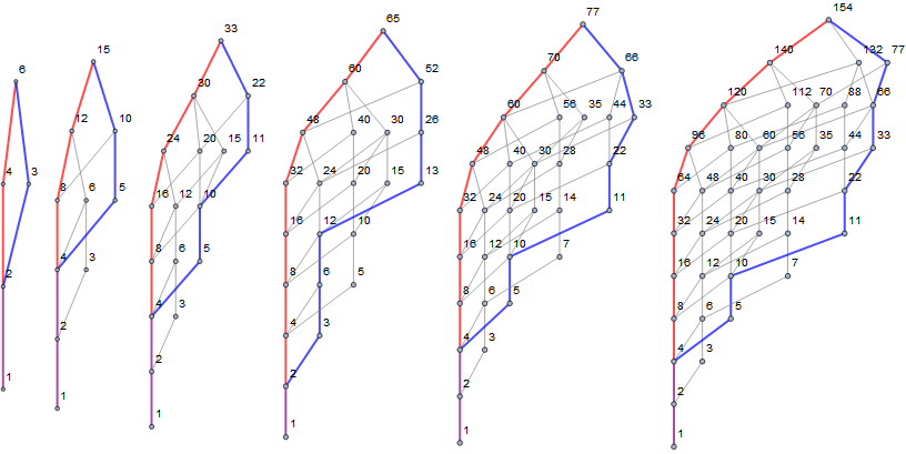
Figure 6 shows lattices for some of the smaller recordsetters in A334144 (Click here for a more expansive montage of lattices for maxima, and here for a montage of the first appearance of w, i.e., terms 2-31 of A333959):
Patterns in the plot of A334144.
We have seen numbers n with total order include the perfect powers of 2 and the Fermat primes; these have w' = a(n) = 1. These appear in the plot as the lowest row of points and are easily explained. Is there any pattern to those n with w' = 2?
Using dataset s = values of A334144 for 1 ≤ n ≤ 10000, we use Position[s, 2][[All, 1]], to obtain their indices n, delimiting them by the perfect powers 2i, and derive the following:
0 | . (null)
1 | .
2 | 6 7
3 | 9 10 11 12 13 14
4 | 18 19 20 22 23 24 25 26 27
5 | 34 40 41 48 50
6 | 68 80 82 83 96 97
7 | 136 137 160 192 193 194
8 | 272 274 289 320 384 386
9 | 514 544 578 640 641 768 769
10 | 1028 1088 1280 1282 1283 1536 1538
11 | 2056 2176 2560 3072
12 | 4112 4352 5120 6144
Mapping (n − 2i) to all of the terms we have:
0 | .
1 | .
2 | 2 3
3 |
1 2 3 4 5 6
4 | 2 3 4 6 7 8 9 10 11
5 | 2 8 9 16 18
6 | 4 16 18 19 32 33
7 | 8 9 32 64 65 66
8 | 16 18 33 64 128 130
9 | 2 32 66 128 129 256 257
10 | 4 64 256 258 259 512 514
11 | 8 128 512 1024
12 | 16 256 1024 2048
These numbers have the following binary weights:
0 | .
1 | .
2 | 2 3
3 | 2 2 3 2 3 3
4 | 2 3 2 3 4 2 3 3 4
5 | 2 2 3 2 3
6 | 2 2 3 4 2 3
7 | 2 3 2 2 3 3
8 | 2 3 3 2 2 3
9 | 2 2 3 2 3 2 3
10 | 2 2 2 3 4 2 3
11 | 2 2 2 2
12 | 2 2 2 2
By this observation, we might be inclined to investigate binary weight in the plot (1 ≤ n ≤ 210) (click here for an expanded plot):

Figure 7 above shows that binary weight is not conserved by a(n). [4]
The most noticeable pattern seems to be the "density striations" that seem to have decreasing slope as n increases. This remains unexplained.
Oscillating Hasse diagrams.
The Hasse diagrams show that the antichains have cardinalities that increase and decrease more than once in certain cases. For 1 ≤ n ≤ 1000, the following numbers have oscillating rank levels [i.e., A334238]:
{57, 63, 171, 258, 266, 294, 301, 329, 342, 343, 354, 361, 377, 378, 379, 381, 387, 399, 423, 437, 441, 462, 463, 469, 474, 481, 483, 489, 506, 513, 529, 567, 603, 621, 642, 643, 689, 798, 817, 889, 903, 931, 978}
Figure 8 shows Hasse diagrams that illustrate the smallest 4 of these oscillating Wichita lattices (see the smallest 24 here):

For terms m at indices i ≤ 710 in A334238, the number of oscillations is 2, meaning that we have figures in row m of A334184 that strictly increase, then decrease, then increase, then decrease, e.g., <><>. These are strictly bimodal, so to speak. Are there terms m in A334238 that have more than 2 oscillations?
Population analysis of A334184.
Consider the sequence A334184, the rank levels w of antichains Aj in the poset P(n), e.g., the “widths” of each “row” of nodes in any of the above Hasse diagrams in Figure 8. For P(57), row 57 of A334184 is {1, 2, 3, 2, 3, 2, 2, 1, 1}, whose total is A332809(57) = 17 nodes, each distinct; the largest value of this row A334144(57) = 3. We now examine the frequency of each term in row n of A334184. In the case of row 57, we have 3 ones, 4 twos, and 2 threes, which we might note m instances of k at position k of a new irregular table t(57) = {3, 4, 2}. Here, we note that, for n that is a Fermat prime 2i + 1, or a perfect power 2i, we have a single term (i + 2) in the case of the former, (i + 1) in the case of the latter, since we have total order in P(n). In other cases we have the following via Code 1.9:
1: 1
2: 2
3: 3
4: 3
5: 4
6: 3 1
7: 4 1
8: 4
9: 4 1
10: 4 1
11: 5 1
12: 3 2
13: 4 2
14: 3 3
15: 3 2 1
16: 5
17: 6
18: 3 3
…
87: 3 3 . 4
88: 4 3 2
89: 5 3 2
90: 3 1 2 2 1
91: 3 3 . 1 3
92: 4 3 3
93: 3 2 1 3 1
94: 4 4 3
95: 3 2 1 2 2
96: 3 5
97: 4 5
98: 3 3 1 3
99: 3 2 1 1 2 1
…
Figure 9 is a heat map where the chroma and intensity of the image portrays the population of terms k in row n of A334184, plotted at (n, k) for 1 ≤ n ≤ 128:

Click to see a larger image in color for 1 ≤ n ≤ 4096, with 16× vertical exaggeration, or in grayscale, for 1 ≤ n ≤ 10000, with 24× vertical exaggeration.
The following table shows the least row n in A334184 where we first find k copies of m. For instance, we first see 5 copies of 4 at row 879 of A334184 = [1, 2, 4, 4, 4, 5, 4, 4, 3, 3, 2, 2, 1, 1]. This shows all n less than or equal to 10000.
k
1 2 3 4 5 6 7 8 9 10
------------------------------------------------------------------------------------
1 | 1 2 6 7 11 34 137 514
2 | 30 15 21 38 106 166 388 771 1546 2566
3 | 35 33 60 114 236 582 908 3592 4614
4 | 65 69 93 129 879 1928 3845 3849
5 | 105 77 264 520 1351 5392 5383
6 | 215 154 161 762 4236
7 | 209 215 429 1197 6498
8 | 319 231 725 2774
9 | 429 385 649 2429
10 | 462 627 667 1251
11 | 469 473 924 2478
12 | 483 693 966 4326
13 | 805 973 2869 3493
14 | 957 987 2065 4731
15 | 1397 1349 3113 3781
16 | 1155 1419 2655 3149
m 17 | 1449 2233 2697 3933
18 | 1463 2001 5607
19 | 2343 2717 2765
20 | 2795 2093 2967
21 | 2093 4085 9373
22 | 3003 2415 3059
23 | 3059 3003
24 | 4186 4389
25 | 4277 6097
26 | 4277 5005
27 | 4899 7029
28 | 4935 7095
29 | 6083 4991
30 | 7161 6149
31 | 6251 6279
32 | 7315 8987
33 | 9177 9869
34 | 9982
This table aims to determine the patterns in the linked enlargements above (after Figure 9) but also visible in Figure 10 that show cusps of high repetition in certain rows:

Indegree and Outdegree.
For each node m in P(n), there are a number of indegrees and a number of outdegrees. In the Hasse diagrams, the indegrees are those chains descending to nodes from above, while the outdegrees are those chains that descend from nodes their children.
Figure 10 shows the indegrees and color codes the nodes as to the number of indegrees. The maximum indegree in each diagram can be found at A332999(n) for n = {15, 57, 119, 210}, i.e., 3, 3, 3, and 4 respectively.

Figure 11 shows the outdegrees and color codes the nodes as to their number. The maximum outdegree in each diagram can be found at A332992(n) for n = {15, 57, 119, 210}, i.e., 2, 2, 3, and 4, respectively.

Code 1.1: In Wolfram language we generate lists of results via the recursive function f(n) = n → n − n/p with prime p|n, with n = 15. In each totally ordered list, the terms mj > m(j + 1), with 0 ≤ j ≤ ℓ. All lists constitute chains and have the common length ℓ = A064097(n):
With[{n = 15}, NestWhile[If[
Length[#] == 0,
Map[{n, #} &, # - # /FactorInteger[#][[All, 1]] ],
Union[Join @@ Map[
Function[{w, n}, Map[
Append[w, If[n == 0, 0, n - n/#]] &,
FactorInteger[n][[All, 1]] ]] @@ {#, Last@ #} &, #]] ] &, n,
If[ListQ[#], AllTrue[#, Last[#] > 1 &], # > 0] &]]
Code 1.2: Use anonymous memoization to generate all chains C for P(n) with 1 ≤ n ≤ 16:
Nest[Function[{a, n}, Append[a,
Join @@ Table[Flatten@ Prepend[#, n] & /@ a[[n - n/p]], {p, FactorInteger[n][[All, 1]]}]]] @@
{#, Length@ # + 1} &, {{{1}}}, 16]
Code 1.3: Simple greatest-to-least sorted tree plots, Hasse diagrams of posets P(n) with 1 ≤ n ≤ 16, here called “Wichita lattices”:
Table[TreePlot[Reverse@ Union@
Apply[Join, #1 -> #2 & @@ # & /@ Partition[#, 2, 1] & /@
NestWhile[If[
Length[#] == 0,
Map[{n, #} &, # - # /FactorInteger[#][[All, 1]] ],
Union[Join @@ Map[
Function[{w, n}, Map[
Append[w, If[n == 0, 0, n - n/#]] &,
FactorInteger[n][[All, 1]] ]] @@ {#, Last@#} &, #]] ] &, n,
If[ListQ[#], AllTrue[#, Last[#] > 1 &], # > 1] &]],
Automatic, n, VertexLabels -> Automatic], {n, 2, 16}] ]
Code 1.4: Generate a montage of Wichita lattices highlighting chains with greatest sums (A333794) in red, those with least sums (333790) in blue, where they are coincident in purple, for posets P(n) with 2 ≤ n ≤ 211. Note: change the variable sort to 0 if least-to-greatest antichain order desired:
Block[{j = 15, k = 24, sort = 1, s, m, mm},
s = Nest[Function[{a, n}, Append[a, Join @@ Table[Flatten@ Prepend[#, n] & /@ a[[n - n/p]],
{p, FactorInteger[n][[All, 1]]}]]] @@ {#, Length@ # + 1} &, {{{1}}}, 14 j + 1];
m = Map[Max[Length@ Union@ # & /@ Transpose@ #] &, s]; mm = Max@ m + 1;
ImageAssemble[Partition[#, j, j], "Fit", Background -> White, Spacings -> 12] &@
Rest@ MapIndexed[Function[{w, n}, Function[{a, b, c, d}, Rasterize@TreePlot[Map[Which[
And[MemberQ[b, #], MemberQ[c, #]], Style[#, Purple, Thickness[1/(k m[[n]])]],
MemberQ[b, #], Style[#, Blue, Thickness[1/(k m[[n]])]],
MemberQ[c, #], Style[#, Red, Thickness[1/(k m[[n]])]],
MemberQ[d, #], Style[#, Green, Thickness[1/(k m[[n]])]],
True, Style[#, Gray]] &, a], Automatic, n,
VertexLabels -> Automatic, DataRange -> {{0, m[[n]]/mm}, {0, 1}},
ImageSize -> Medium] ] @@
{If[sort == 1, Reverse@ #, #] &@
Union@ Apply[Join, #1 -> #2 & @@ # & /@ Partition[#, 2, 1] & /@ #1],
#1 -> #2 & @@ # & /@ Partition[#1[[FirstPosition[#2, Min@ #2][[1]] ]], 2, 1],
#1 -> #2 & @@ # & /@ Partition[#1[[FirstPosition[#2, Max@ #2][[1]] ]], 2, 1],
#1 -> #2 & @@ # & /@ Partition[
NestWhileList[# - #/FactorInteger[#][[-1, 1]] &, n, # > 1 &], 2, 1]
} & @@ {w, Total /@ w}] @@ {#1, First@ #2} &, s ] ]]
Code 1.5: Generate A333123 for 1 ≤ n ≤ 105:
Nest[Append[#1, Sum[#1[[#2 - #2/p]], {p, FactorInteger[#2][[All, 1]]}]] & @@
{#, Length@ # + 1} &, {1}, 120] ]
Code 1.6: Generate A334144 for 1 ≤ n ≤ 105:
Monitor[Table[Max[Length@ Union@ # & /@ Transpose@ #] &@
If[n == 1, {{1}}, NestWhile[If[Length[#] == 0,
Map[{n, #} &, # - # /FactorInteger[#][[All, 1]] ],
Union[Join @@ Map[Function[{w, n}, Map[Append[w, If[n == 0, 0, n - n/#]] &,
FactorInteger[n][[All, 1]] ]] @@ {#, Last@ #} &, #]]
] &, n, If[ListQ[#], AllTrue[#, Last[#] > 1 &], # > 1] &]], {n, 105}], n]
Code 1.7: Generate A334184 for 1 ≤ n ≤ 22:
Map[Map[Length@ Union@ # &, Transpose@ #] &,
Nest[Function[{a, n}, Append[a, Join @@ Table[
Flatten@ Prepend[#, n] & /@ a[[n - n/p]], {p, FactorInteger[n][[All, 1]]}]]] @@
{#, Length@ # + 1} &, {{{1}}}, 22]]]
Code 1.8: Generate m in A333259 with m ≤ 1000:
With[{s =
Table[Max[Length@ Union@ # & /@ Transpose@ #] &@
If[n == 1, {{1}}, NestWhile[If[Length[#] == 0,
Map[{n, #} &, # - # /FactorInteger[#][[All, 1]] ],
Union[Join @@ Map[Function[{w, n},
Map[Append[w, If[n == 0, 0, n - n/#]] &,
FactorInteger[n][[All, 1]] ]] @@ {#, Last@ #} &, #]] ] &, n,
If[ListQ[#], AllTrue[#, Last[#] > 1 &], # > 1] &]], {n, 10^3}]},
TakeWhile[Array[FirstPosition[s, #][[1]] &, Max@s], IntegerQ]] ]
Code 1.9: Write the number of instances of the value k in row n of A334184 at position k, with n ≤ 120:
Block[{s = Map[Map[Length@ Union@# &, Transpose@ #] &,
Nest[Function[{a, n}, Append[a, Join @@
Table[Flatten@ Prepend[#, n] & /@ a[[n - n/p]],
{p, FactorInteger[n][[All, 1]]}]]] @@
{#, Length@ # + 1} &, {{{1}}}, 120]] , w},
w = ConstantArray[0, Max@ Flatten@ s];
Map[Reverse@ Drop[#, LengthWhile[#, # == 0 &]] &@
ReplacePart[w, Map[-#1 -> #2 & @@ # &, Sort@ Tally@ #]] &, s]]
Acknowledgements:
The author thanks Peter Kagey for comments and guidance at A334144, regarding combinatorics and set theory. This sequence was written in connection with several related sequences studied by Rémy Sigrist, Robert G. Wilson V, and Antti Karttunen. The sequence arose in conjunction with the author's coding efforts, both in generating terms and plotting Hasse diagrams relating to Antti Karttunen's agency at A333790. Thanks to Robert G. Wilson V for inviting the author and others on the authorship of A333959.
References:
[1] Peter Kagey, “pink box” discussion comment under edit #3 at A334144, Thursday 16 April 2020, 17:57:
This defines a graded poset, and this sequence gives the largest rank level. Are these posets Sperner? If so, then the largest rank level is the largest antichain.
[2] Wikipedia, “Sperner property of a partially ordered set”. Link provided by [1] above.
[3] Richard Stanley, “The Sperner property”. Massachusetts Institute of Technology: MIT OpenCourseWare course 18.318: Topics in Algebraic Combinatorics (spring 2006).
[4] Antti Karttunen, “pink box” discussion comments under edit #10 at A334144, Friday 17 April 2020, 18:46, regarding binary weight.
Concerns sequences:
A019434: Fermat primes: primes of the form 2^(2^k) + 1, for some k ≥ 0.
A064097: Number of iterations of the map f(n) = n → n − n/p with prime p|n necessary to reach 1.
A332809: Number of distinct integers generated by P(n), or nodes in the Wichita lattice of n.
A332992: Maximum outdegree of Wichita lattice P(n).
A332999: Maximum indegree of Wichita lattice P(n).
A333123: Width of Wichita lattice P(n); the number of chains C generated by the recursive function f(n).
A333790: Chain with least sum in the Wichita lattice P(n), shown in blue in figures 2, 3, and 5.
A333794: Chain with greatest sum in the Wichita lattice P(n), shown in red in figures 2, 3, and 5.
A333959: Index m of first instance of n in A334144.
A334144: Largest rank level of all antichains in the poset P(n).
A334184: Rank levels of all antichains in the poset P(n).
A334238: Rows m in A334184 that are not unimodal.
Document Revision Record.
2020 0416 1430 Created.
2020 0416 2200 Records transform extension, typos, larger plot montages.
2020 0417 1000 Records and indices of values of w in A334144(n), 1 ≤ n ≤ 6000.
2020 0418 0800 Incorporates results of 10000 term dataset, language alteration, references, acknowledgements.
2020 0418 1700 Observations regarding binary weight added.
2020 0418 2200 Oscillating Wichita lattices and A334184 added.
2020 0422 1415 Related sequences referenced.
2020 0422 2100 Population analysis of A334184, Code 1.9 added.
2020 0425 1300 Links updated, bimodality of row m of A334184, for m in A334238(i) and i ≤ 710.
2020 0430 1615 In- and outdegrees with diagrams at Figures 10 and 11.
2020 0502 1630 New title (originally, “OEIS A334144”).