OEIS A338209
Written by Michael Thomas De Vlieger, St. Louis, Missouri, 2020 1016.
Abstract.
Consider the binary weight w(n) of the number n, meaning the number of 1 digits (or bits) in the binary expansion of n. Essentially, the binary weight of a number is equivalent to the digit sum of the binary expansion of that same number. We examine 3 integer sequences that begin with the first term set to 1. The succeeding term finds the bits that comprise the binary expansion of the binary weight w of the preceding term somewhere among the bits of the binary expansion of a least novel number m. Sequence a(n) = A338209(n) looks for w among the very final bits of m, while b(n) = A339024(n) the very first, and c(n) = A339607(n) anywhere in the binary expansion of m. This work explores the behavior of each sequence given 16384 terms of each. We find that a(n) relates to a congruence relation whose plot has the character of branching streams associated with the congruences and the binomial distribution of the binary weight of numbers already seen in the sequence. The sequence b(n) looks for w in the most significant bits of m. The plot of b(n) fills families associated with a range of numbers that are part of a rank interval according to perfect powers of 2. The last sequence c(n) looks for the bits that comprise w just as they appear in w anywhere among the bits of m. This sequence does not vary far from the sequence of natural numbers, but the amplitude of c(n) − n does seem to respond to the magnitude of w.The sequences are likely permutations of the natural numbers.
Introduction.
Let us consider 3 related self-referential sequences involving the binary weight w2 (a “word” written in binary) of the previous term governing the presence of the bits w2 somewhere among those in a novel least term m not already in the sequence.
Binary weight.
The binary weight w(n) = OEIS A120 is the number of 1s in the binary expansion of n. Therefore, with 12 → 11002, w(12) = 2 → 102. We abbreviate this function in this work as n ⇒ w2, thus, 728 ⇒ 1012, since 728 in binary is 10110110002. For simplicity, we will drop the subscript from the word w throughout this paper.
Figure 1 is a textual plot of (n, w(n)) for 1 < n < 64:
A120: Binary weight of n o
o o o o oo.
o o o oo. o o oo. o oo. oo.o...
o o oo. o oo. oo.o... o oo. oo.o... oo.o...o.......
o oo. oo.o... oo.o...o....... oo.o...o.......o...............
oo.o...o.......o...............o...............................o
|| | | | | | | | |
12 4 8 16 24 32 40 48 64
The function w(n) has a fractal nature regarding the interval I( j) = 2 j ≤ n ≤ (2( j + 1) − 1), such that we might tally the values k taken by w(n) in these intervals I( j) and derive Pascal's Triangle (A7318) via T( j, k) = binomial( j, k − 1).
Table 1 shows the number of values k taken by w(n) in the interval I( j):
2^j...2^(j+1)-1
1: 1 1 2.....3
2: 1 2 1 4.....7
3: 1 3 3 1 8....15
4: 1 4 6 4 1 16....31
j 5: 1 5 10 10 5 1 32....63
6: 1 6 15 20 15 6 1 64...127
7: 1 7 21 35 35 21 7 1 128...255
8: 1 8 28 56 70 56 28 8 1 256...511
-----------------------------------------
1 2 3 4 5 6 7 8 9
Binary weight k
Table 1 shows us that there is only 1 number in an interval I( j) with the least binary weight k = 1 for n = 2 j, and 1 number in same with greatest binary weight k = j + 1 for 2( j + 1) − 1. Further there are j numbers with k = 2 or j numbers with k = j. The greatest population of binary weight values in the interval appear at the middle of the range of values. Thus, for example, for the interval beginning with 29 = 512, the most common binary weight is 5. The nature of w(n) certainly influences the behavior of the three sequences we shall examine.
The three sequences we consider directs the word w to different positions in m. a(n) directs the word w to the least bits of m; b(n) to the greatest bits of m, and c(n) in any position within the binary expansion of m.
Thus, we define the three sequences:
a(1) = 1; a(n) is the least m not already in a(n) that has the word w(a(n − 1)) as its least significant (i.e., last) bits.
b(1) = 1; b(n) is the least m not already in b(n) that has the word w(b(n − 1)) as its most significant (i.e., first) bits.
c(1) = 0; c(n) is the least m not already in c(n) such that the word w(c(n − 1)) appears anywhere within the binary expansion of m.
The “word → least” sequence.
The first sequence to consider, a(n) = A338209(n), situates the word w = w(a(n − 1)), expressed in binary notation, at the end of the binary expansion of the least m not already in a(n). This is tantamount to finding the least m not already in a(n) such that m mod 2k ≡w(a(n − 1)), where k = ⌊1 + log2 w(a(n − 1))⌋ is the binary word length of w.
Example: we have a(9) = 11 → 10112 ⇒ 3 → 112. We have already seen 3, 7, 11 in the sequence, with binary expansions with the ending 112. The next number not already used is 15 → 11112.
Michael S. Branicky showed that a(n) is a permutation of the integers since n appears at or before index 2n − 1, the first number with binary weight n.
The sequence a(n) begins:
1, 3, 2, 5, 6, 10, 14, 7, 11, 15, 4, 9, 18, 22, 19, 23, 12, 26, 27, 20, 30, 28, 31, 13, 35, 39, 36, 34, 38, 43, 44, 47, 21, 51, 52, 55, 29, 60, 68, 42, 59, 37, 63, 46, 76, 67, 71, 84, 75, 92, 100, 79, 45, 108, 116, 124, 53, 132, 50, 83, 140, 87, 61, 69, ...
(Generate per Code A. Here is an OEIS-style list of n, a(n) with 16384 terms.)
a(n) as a consequence of congruence.
Because we are looking for a binary word w at the least significant end of another binary expansion m ≥ w, given a binary number must begin with the bit 1, and that a perfect power 2e expanded in binary is a 1 followed by e zeros, we find that 2e enters the sequence much later than other numbers of similar magnitude. Also delayed are numbers that end in a long run of zeros.
Is it true that a(n) is a permutation of the natural numbers? It seems true, since a prohibition of the binary weight of a previous term would mean that the number of 1-bits in the binary expansion of the previous term would never occur, something that seems unlikely. It remains unproved.
The numbers 2e with 0 ≤ e ≤ 4 appear at indices {1, 3, 11, 222, 47201}. Given 214 terms, we surmised that 16 may not appear until n ≈ 216, when we have the potential to have an odd m with the maximum binary weight of 16, given the maxima of a(n) generally 2.5 n. Michael S. Branicky found a(47201) = 16. It will require ever greater n to result in w = 2e. Such a w may become “common” for sufficiently large n, with a(n) ≈ 22e, that is, a magnitude that produces numbers more likely to result in a binary weight w = 2e.
The numbers (2e + 1) directly follow terms m = 2(e − 1), since all m such that log2 m is not an integer has binary weight that exceeds 1; only perfect powers of 2 have the binary weight 1. Therefore these appear at indices {2, 4, 12, 223, …}, and we should see the term 33 following 32. As we generate terms in a(n), terms (2e + 1) are the longest-missing from the sequence.
The numbers (2e − 1) with 1 ≤ e ≤ 14 appear at indices {1, 2, 8, 10, 23, 43, 130, 278, 447, 758, 1390, 2525, 4719, 9333}.
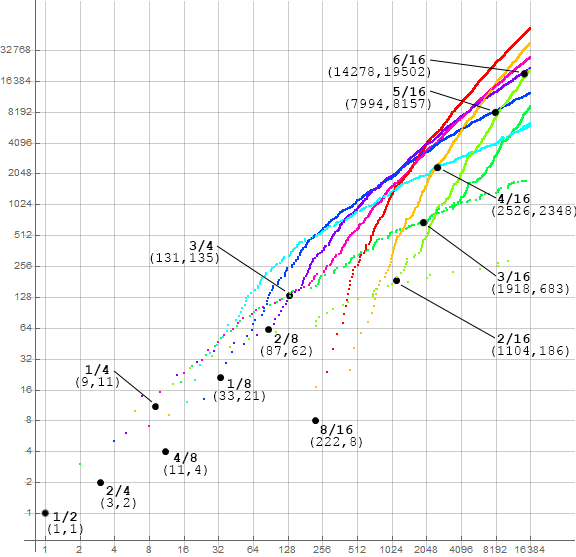
Figure A1: plot of a(n) for 1 ≤ n ≤ 4096 reveals a principal feature of the sequence: streams of a(n) ≡ r (mod 2k). (see Code A1):

Arrangement of a(n) into dendritic streams of residues.
The result of searching for the least m not already in a(n) such that m mod 2k ≡ w is the dendritic division of the plot into streams of residues r (mod 2k).
Figure A2 shows the first 256 terms, many labeled automatically. We color these in terms of their residue r (mod 8). The residue 0 in red, +1 in gold, +2 in yellow-green, +3 in true green, 4 in cyan, −3 in blue, −2 in violet, and −1 in magenta. We see that the residues +3 and −1 appear to decouple at n = 128, and ±2 around n = 32. (See Code A2)

Figure A3 shows 212 = 4096 terms with the same color scheme. We see that the residues 0 and +1, though they seem to have gotten a late start, eventually become as prominent as the other lines. The residue 0 ends up setting records. (See a magnified plot of a(n) for 1 ≤ n ≤ 214.)

Do the 8 prominent streams divide, perhaps so as to be r (mod 16), much as they seemed to have done from r (mod 4) at n = 32 and n = 128?
In the examination of the extended plot, we indeed see a decoupling according to r (mod 16), at least for some streams. Let the term “pitch” δ denote the first differences of the “stream” of terms m ≡ r (mod 2k). We note that the stream plotted in red for m ≡ 0 (mod 8), {8, 24, 40, 56, 72, …}, does not share the pitch δ = 8 that we see in other streams. Instead it has δ = 16 and thus, already can be construed as m ≡ 8 (mod 16).
We might divide a(n) into various streams ς, denoted by their congruence r (mod 2⌊1 + log2 n⌋. Thus we have ς(8/16, n) = {8, 24, 40, 56, 72, …}.
We can locate the decoupling of ς(3/4, n) = {3, 7, 11, 15, 19, 23, 27, 31, …} into ς(3/8, n) shown in purple in Figures A2 and A3, and ς(7/8, n) shown in yellow green. Indeed, these appear such that the first differences of their indices is always positive until (n, a(n)) = (131, 135). Certainly we see decoupling with 151 at a(150), 155 delayed to a(202) after a(176) = 159.
Similarly, we find the decoupling of ς(4/8, n) = {4, 12, 20, 28, 36, 44, …} into ς(4/16, n) and ς(12/16, n). The split takes place among 12 (mod 16) ≡ 2332 at a(2515), 2340 delayed to a(2533) after a(2526) = 2348.
We also find the decoupling of ς(2/4, n) = {2, 6, 10, 14, 18, 22, 26, …} into ς(2/8, n) and ς(6/8, n). The split takes place among 6 (mod 8) ≡ 54 at a(69), 58 delayed to a(102) after a(87) = 62.
Figure A4 shows the descent of streams ς according to their decoupling. The numbers in red are forbidden, since they pertain to w = 0 which is not permitted since 0 is not in a(n). We have ς(1/2, n) at level 1 (which contains only m = 1), then at level 2 we have ς(1/4, n) and ς(3/4, n) descend from ς(1/2, n), while ς(2/4, n) arises with a(3) = 2.
At level 3 we have ς(1/4, n) give rise to ς(1/8, n) with a(223) = 17, and ς(5/8, n) with a(33) = 21. We can also find ς(2/4, n) → {ς(2/8, n), ς(6/8, n)}, ς(3/4, n) → {ς(3/8, n), ς(7/8, n)}. while ς(4/8, n) arises with a(11) = 4.
At level 4 we have divisions as shown, while ς(4/8, n) arises with a(222) = 8.
Figure A4. OEIS A049773, relating to the division and introduction of streams branching from those in a level above it in the graph. Read each number as r (mod k), where r is in a white bubble, and k is the red bubble directly to its right. In other words, we regard the numbers in white as r (mod 2ℓ), where ℓ is the base-2 logarithm of the number of terms in the level. (See an expanded chart to ℓ = 6.)

Table A1 lists the points of bifurcation of the stream designated at left, or the introduction of the stream. For example, ς(3/4, n) → {ς(3/8, n), ς(7/8, n)} occurs at a(131) = 135 ≡ 7 (mod 8).
1/2 -> (1/4, 3/4): a(9) = 11
Introduce 2/4 : a(3) = 2
1/4 -> (1/8, 5/8): a(33) = 21
3/4 -> (3/8, 7/8): a(131) = 135
2/4 -> (2/8, 6,8): a(87) = 62
Introduce 4/8 : a(11) = 4
1/8 -> (1/16, 9/16): ?
5/8 -> (5/16, 13/16): a(7994) = 8157
3/8 -> (3/16, 11/16): a(1918) = 683
7/8 -> (7/16, 15/16): ?
2/8 -> (2/16, 10/16): a(1104) = 186
6/8 -> (6/16, 14/16): a(14278) = 19502
4/8 -> (4/16, 12/16): a(2526) = 2348
Introduce 8/16 : a(222) = 8
Figure A5 is a log2-log2 plot of a(n) for 1 ≤ n ≤ 214 using the same color code as Figures A2 and A3 showing the coordinates (n, a(n)) where ς splits into the listed designation and its complement.
Can we truly have a stream that contains numbers congruent to 0 (mod 2k), or are these really 2k (mod 2(k + 1))? A stream with a(n) ≡0 (mod 2k) implies w = 0 which is not seen outside of a(n − 1) = 0, and would be resolved by any available even m. Since the sequence does not begin with 0, we will not see w = 0. Therefore we shall construe the apparent stream of a(n) ≡0 (mod 2k) instead as 2k (mod 2(k + 1)). This is corroborated by the observation of the streams ς(2/4, n), ς(4/8, n) and ς(8/16, n).
We may then find the indices of the first terms of positive residue r in a(n):
1, 3, 12, 9, 448, 87, 131, 222, …
What causes the division of streams r (mod 2k) into r (mod 2(k + 1)) and (r + 2k) (mod 2(k + 1))? For example, the numbers 3 (mod 4) have “11” as the last bits of their binary expansion, and at some point, the stream divides into numbers congruent to 3 (mod 8) ending in “011” and 7 (mod 8) ending in “111”. Similarly, those numbers congruent to 4 (mod 8) ending in “100” are divided into numbers congruent to 4 (mod 16) ending in “0100”, and 12 (mod 16) ending in “1100”. Therefore, what we are saying when we speak of a division of streams, is that we are no longer seeking k-bit suffixes, but now (k + 1)-bit suffixes. This implies that we have exhausted suffixes that have a given configuration of k bits, and now must find that configuration as the final k bits of an (k + 1)-bit suffix, prepending a 0 or a 1 bit to that original k-bit suffix. The division of suffixes implies that the lengthened suffix (r + 2k) (mod 2(k + 1)) richer in 1-bits is preferred over r (mod 2(k + 1)) with fewer 1s.
Is it true that we see ever larger w, and always see w of any magnitude less than ⌊1 + log2 n⌋ where there is potential to have m with the binary weight ⌊1 + log2 n⌋? We know w = 1 becomes rare, marking the position of perfect powers of 2 in a(n).
For instance, we see w = 2 instigated by a(223) = 17, after an absence since a(101) = 260. In the description below, we delimit the bits of w found in the binary expansion of m using a dot:
8 → 12 ⇒ 17 → 100012 ⇒ 2 → 102: 66 → 10000.102 ⇒ 2 → 102: 74 → 10001.102 ⇒ 3 → 112.
The number 17 = 2e + 1 follows 2e in a(n), therefore is a late-comer; the number w = 2 is occurs relatively infrequently (i.e., 2 occurs j times within the interval I( j) = 2 j ≤ n ≤ (2( j + 1) − 1) ). Here we see a(223) = 17 = ς(1/8, 3) lead to a(224) = 66 = ς(2/8, 9), then to a(225) = 74 = ς(2/8, 10).
The indices in a(n) with binary weight w = 2, we have:
2, 4, 5, 6, 12, 13, 17, 20, 27, 28, 39, 58, 101, 223, 224, 236, 279, 318, 383, 426, 522, 698, 699, 716, 942, 1411, 2081, 2195, 3492, 5926, 8559, 8560, 10521, ...
The numbers a(n + 1) that result from these belong to 2 (mod 4), and after a(69...102), 2 (mod 8), thus prefering the stream closest to the x-axis in Figure A2. While ς(2/4, n) is running to the split at a(69) = 54, the terms a(n + 1) include every m (mod 2) and m (mod 6) except a(44) = 46 ≡6 (mod 8). We see 63 → 1111112 ⇒ 1102: 46. Thereafter, w = 2 takes m ≡ 2 (mod 8) and never m ≡ 6 (mod 8).
Furthermore, numbers m ≡ {2, 10} (mod 16) are instigated by w = 2 for n ≤ 699, but a(759) = 154 ≡ 10 (mod 16), but is instigated instead by w = 10. At some point we should see a division ς(2/8, n) into ς(2/16, n) and ς(10/16, n), but for n ≤ 214, the two streams are still unified.
Therefore we witness perhaps, the division of ς(2/4, n) into ς(2/8, n) initially predominated by 2 ⇒ m and ς(6/8, n) initially predominated by even w > 2 ⇒ m. Then in ς(2/8, n) we have 2 ⇒ m along with other w ≡ 2 (mod 8).
These questions remain to be answered and the answers proved, however it seems that once we have a k-bit stream ς, we can find all w with fewer bits (i.e., shorter word lengths) that represent a truncation of the leftmost bits of ς within stream ς. Furthermore, such truncated w prefer to find m in “lower” streams ς. This suggests the streams will never re-merge but instead remain separate after branching unless perhaps they dither while in the process of branching.
Figure A6 is a log2-log2 plot of a(n) for 1 ≤ n ≤ 214 using the same color code as Figures A2 and A3 highlighting the records described above:

The maxima of a(n).
We do see certain streams dominating the maxima of a(n). ς(4/8, n) generally sets records between a(38) = 60 and a(182) = 468. There is a transition zone with first differences in the maxima moving from solidly 8 through {1, 7, 8, 1, 7, 1} to the next phase of maxima, with ς(5/8, n) setting records between a(215) = 493 through a(834) = 1645. A second transition with first differences moving through {1, 7, 1, 8, 7, 8, 8, 1} separates this phase from one where ς(6/8, n) sets records between a(865) = 1686 and a(2039) = 3910. A third transition with first differences in the maxima moving from solidly 8 through {2, 6, 10} to solidly 16. Finally, ς(8/16, n) sets records beginning with a(2048) = 3928. From an expanded log2-log2 plot of a(n) accentuating maxima, we see that perhaps the streams never re-merge. This remains to be proved.
The effect of repeated w on the plot of a(n).
We may generate an auxiliary sequence wa(n) that notes the binary weight w that instigates the term a(n). This sequence begins:
1, 2, 1, 2, 2, 2, 3, 3, 3, 4, 1, 2, 2, 3, 3, 4, 2, 3, 4, 2, 4, 3, 5, 3, 3, 4, 2, 2, 3, 4, 3, 5, 3, 4, 3, 5, 4, 4, 2, 3, 5, 3, 6, 4, 3, 3, 4, 3, 4, 4, 3, 5, 4, 4, 4, 5, 4, 2, 3, 4, 3, 5, 5, 3, ...
From wa(n), we take run lengths and map them to each term to derive the sequence ℓa(n):
1, 1, 1, 3, 3, 3, 3, 3, 3, 1, 1, 2, 2, 2, 2, 1, 1, 1, 1, 1, 1, 1, 1, 2, 2, 1, 2, 2, 1, 1, 1, 1, 1, 1, 1, 1, 2, 2, 1, 1, 1, 1, 1, 1, 2, 2, 1, 1, 2, 2, 1, 1, 3, 3, 3, 1, 1, 1, 1, 1, 1, 2, 2, 1, ...
From this we can produce a plot like Figure A2 that shows where we have repeated invocations of the same binary weight w.
Figure A7 shows the first 256 terms of a(n), showing terms arising from singleton w in small green dots, terms arising from the same back-to-back w in medium blue dots, and triplicated invocations of w in large red dots, some of which are automatically annotated. We see that the difference between these red dots is 8; indeed the same is true for the duplicated blue dots.

Depiction of terms of a(n) as a bitmap.
Figure A8 depicts a(n) in binary, with black = 1 and white = 0, starting with a(1) = 1 at left, vertically, the least bit at bottom, running through a(256) = 556 → 10001011002 at right.
![]()
Figure A9 depicts a(n) in binary, with black = 1 and white = 0, starting with a(1) = 1 at left, vertically, the least bit at bottom, running through a(1024) = 313 → 1001110012 at right.
![]()
Conclusion.
A sequence akin to this one in decimal, but pertaining to decimal digital roots, is explained in another paper, there called the “root-least” sequence, OEIS A338191.
The sequence is a permutation of the natural numbers. We can find binary weights 0 < w(n) for any binary number n > 0, though some numbers are more reluctant to enter the sequence on account of their having many trailing zeros. The sequence a(n) is characterized by dendritic “streams” of m ≡r (mod 2k). The reason for the division of the plot into branching streams and whether or not the streams re-merge remain unanswered questions.
The “word → most” sequence.
The sequence b(n) situates the word w = w(b(n − 1)) i.e., the binary weight of the preceding term, expressed in binary notation, in the most significant bits of the binary expansion of the least m not already in a(n). In other words, the bits in w are a prefix in the binary expansion of m. It begins:
1, 2, 3, 4, 5, 8, 6, 9, 10, 11, 7, 12, 16, 13, 14, 15, 17, 18, 19, 24, 20, 21, 25, 26, 27, 32, 22, 28, 29, 33, 23, 34, 35, 30, 36, 37, 31, 40, 38, 48, 39, 64, 41, 49, 50, 51, 65, 42, 52, 53, 66, 43, 67, 54, 68, 44, 55, 45, 69, 56, 57, 70, 58, 71, ...
Generate per Code B. Since there are often large first differences in this sequence as n increases, it is the most difficult of the three for which to generate a large amount of terms. (Here is an OEIS-style list of n, b(n) with 16384 terms)
b(2) = 2 since the binary weight of b(1) = 1 is 1, and we find a “1” at the beginning of the binary expansion of the succeeding m = 2.
b(3) = 3 since the binary weight of b(2) = 2 is 1, and we find a “1” at the beginning of the binary expansion of the succeeding m = 3.
b(4) = 4 since the binary weight of b(3) = 3 is 2, which is written “10” in binary. We find that the succeeding m = 4 starts with “10” when expanded in binary.
b(5) = 5 since the binary weight of b(4) = 4 is 1, and we find a “1” at the beginning of the succeeding m = 5 expressed in binary.
b(6) = 8 since the binary weight of b(5) = 5 is 2, which is written “10” in binary. We find that the succeeding m = 6 starts with “11” in binary, as does m = 7. Only when we reach m = 8 do we find a binary number that begins with “10”.
b(7) = 6 since the binary weight of b(6) = 8 is 1, and we find a “1” at the beginning of the least unused number m = 6 expressed in binary.
b(8) = 9 since the binary weight of b(7) = 6 is 2, which is written “10” in binary. We find that the least unused m = 7 starts with “11” in binary, and m = 8 is used. Only when we reach m = 9 do we find an unused binary number that begins with “10”.
etc.
Michael S. Branicky showed that b(n) is a permutation of the integers since n appears at or before index 2n − 1, the first number with binary weight n.
The resultant sequence b(n) is organized into streaky clouds in a “family” that is a range M(i) ≤ m < M(i + 1) whose binary expansion begins with an odd number “prefix” m/2v, where v is the 2-adic valuation of m. (There are thus 2v numbers in this range.) The numbers in this range accommodate the binary weights 1 ≤ w ≤ ⌈log2 b(n − 1)⌉ of the previous term b(n − 1) such that the binary expansion of w appears in part or all of the binary expansion of the prefix m/2v, and perhaps an additional bit in m after the prefix. Small values of w, for instance w = 1, may appear in any family, but large w require the entire prefix and potentially more (if even). The w that cannot be found in a particular family are found in a different family that has M(i + 1) as its least member. At some point, all the numbers in the range m are exhausted, and in order to obtain the same prefix m/2v, we increment v so as to furnish a new font of m that might accommodate w. In these cases, w tends to be large.
Therefore, the plot obeys an arrangement that features these ranges in various overlying quasi-linear “clouds” wherein b(n) is populated among several as n increases, exhausting the lesser families and engaging greater ones as necessary.
Figure B1 is a plot of the first 4096 terms of b(n), showing the clouds in streaks associated with families of consecutive numbers that are a prominent feature of the sequence (see Code B1):

Arrangement of terms in b(n) into families and classes.
This plot shows the exhaustion of numbers that begin with a given binary word w, with the function jumping an order of magnitude to w × 2(e+ 1) + j once we have depleted all w × 2e + j. At some point all 2e ≤ m < 2(e+ 1) are in b(n).
Figure B2 labels (n, b(n)) for many of the points, automatically, for 1 ≤ n ≤ 128. Numbers b(n) that are perfect powers of 2 appear in red, while those that are the sum of two perfect powers of 2 are shown in gold. Even b(n) are in light blue while odd are in black. (See Code B2).

Figure B3 plots the first 4096 terms, accentuating b(n) that are perfect powers of 2 in red, and the sums of two perfect powers of 2 in gold, labeling (n, b(n)) for some perfect powers of 2:

We see that b(n) exhibits meteor-like “streaks” we will call families herein, that begin with a number m in a series M(i) that includes perfect powers of 2:
{1, 2, 4, 8, 16, 24, 32, 40, 48, 64, 80, 96, 128, 160, 192, 224, 256, 320, 384, 448, 512, 640, 768, 896, 1024, 1152, 1280, 1536, 1792, 2048, 2304, 2560, 2816, 3072, 3584, 4096, 4608, 5120, 5632, 6144, 7168, 8192, 9216, 10240, 11264, 12288, 13312, 14336, 16384, 18432, 20480, …}
Truncating the rightmost run of zeros from these numbers m that are even except 1, we obtain odd m/2v, where v is the 2-adic valuation of m. In terms of the OEIS:
m/2v = m/2A7814(m)
Table B1 lists the numbers in family M(i) along with their 2-adic valuation or “class” M(i)/2v and their binary expansions:
i Family Rank Class M(i)_2
------------------------------------
1 1 0 1 1
2 2 1 1 10
3 4 2 1 100
4 8 3 1 1000
5 16 4 1 10000
6 24 3 3 11000
7 32 5 1 100000
8 40 3 5 101000
9 48 4 3 110000
10 64 6 1 1000000
11 80 4 5 1010000
12 96 5 3 1100000
13 128 7 1 10000000
14 160 5 5 10100000
15 192 6 3 11000000
16 224 5 7 11100000
17 256 8 1 100000000
18 320 6 5 101000000
19 384 7 3 110000000
20 448 6 7 111000000
21 512 9 1 1000000000
22 640 7 5 1010000000
23 768 8 3 1100000000
24 896 7 7 1110000000
25 1024 10 1 10000000000
26 1152 7 9 10010000000
27 1280 8 5 10100000000
28 1536 9 3 11000000000
29 1792 8 7 11100000000
30 2048 11 1 100000000000
31 2304 8 9 100100000000
32 2560 9 5 101000000000
33 2816 8 11 101100000000
34 3072 10 3 110000000000
35 3584 9 7 111000000000
36 4096 12 1 1000000000000
37 4608 9 9 1001000000000
38 5120 10 5 1010000000000
39 5632 9 11 1011000000000
40 6144 11 3 1100000000000
41 7168 10 7 1110000000000
42 8192 13 1 10000000000000
43 9216 10 9 10010000000000
44 10240 11 5 10100000000000
45 11264 10 11 10110000000000
46 12288 12 3 11000000000000
47 13312 10 13 11010000000000
48 14336 11 7 11100000000000
49 16384 14 1 100000000000000
50 18432 11 9 100100000000000
51 20480 12 5 101000000000000
...
Let k = ⌊1 + log2 M(i)⌋. Therefore we may designate the family M(i)/2v × 2(k − v) + j beginning with M(i) as the family of M(i). We may say that the families with the same M(i)/2v belong to the same class M(i)/2v. The sequence b(n) finds w in the family, matching the most significant bits of w with those in the binary expansion of M(i)/2v along with additional bits as necessary in M(i) × 2(k − v) + j, (normally zeros).
For example, b(79) = 63 gives rise to the family of 96:
b(79) = 63 → 11.11112 ⇒ 6 → 1102: 96 → 110.000002
The next term that needs a number beginning with the bits “11”:
b(86) = 84 → 1.0101002 ⇒ 112: 97 → 11.0000012
We see that, in the case of b(79) = 63, which is the last term of the family 48 preceding the next family, 96, in the same class 3. This coterminal situation is not always the case: 127 = b(197) is the last term of family 96, but occurs after the first term of family 192, b(132) =192.
As to classes, there are 6 observed in b(n) for n ≤ 8192. Within these classes we observe w such that the binary expansion of w begins with the first bits or all of the bits of M(i)/2v, and sometimes some bits that follow within the family. Class 1 includes all w whose binary expansions start with 1 and thereafter have trailing zeros, i.e., 1, 2, 4, 8, …; therefore class 1 includes w that are perfect powers of 2.
Table B2 lists the classes with the binary expansion of their prefixes, followed by w seen in the class, and OEIS sequences likely to be subsets of the class (See this expanded table that concatenates w seen in the smallest families of the given classes):
Class Binary w seen in class Includes OEIS
------------------------------------------------------
Class 1: 1...: 1, 2, 4, 8, ... A000079
Class 3: 11...: 1, 3, 6, ... (A003945)
Class 5: 101...: 1, 2, 5, 10, ... (A020714)
Class 7: 111...: 1, 3, 7, ... (A005009)
Class 9: 1001...: 1, 2, 4, 9, ... (A005010)
Class 11: 1011...: 1, 5, 11, ... (A118413 row 6)
Class 13: 1101...: 1, 6, 13, ... (A118413 row 7)
Class 15: 1111...: 1, 3, 7, 15, ... (A118413 row 8), A000225
...
We anticipate a class 13 → 11012 and 15 → 11112. At a certain point, we will have classes pertaining to odd numbers greater than 16 as well, just as we have class 9 materialize for n = 1125. Class 17 will appear once we require a binary weight of 17, that is, when b(n − 1) = 262143. We find 2k − 1 at the following indices:
1, 3, 11, 16, 37, 79, 197, 428, 811, 1395, 2539, 4750, 9180, ...
Furthermore, w is very often repeated, unlike the case of seldom-repeated w in the “word→least” sequence a(n).
Are there even classes, or are all the needs for finding even w met by the first half of the odd classes? Indeed, half of the numbers in a family of class M(i)/2v. Therefore it does not seem that there are even classes, and that the odd classes accommodate even w either as a left-trim portion of the prefix M(i)/2v, or via a zero-bit appended to the prefix. An example of a situation where even w is required of a class M(i) with a smaller bit length than w is n = 17. For n = 17, w(b(n − 1)) = w(15) = 4, but the family where the solution (17) is found is that of 16, which is 1 × 24.
Coincidentally, we find n = b(n) in increasingly few places:
1, 2, 3, 4, 5, 12, 17, 18, 19, 28, 29, 54, 173, 174, 175, 199, 225, 417, 736, 862, 1903, 2739, 4341, 4656, 13336, ...
We see that, whereupon all the terms M(i) ≤ m ≤ M(i + 1) − 1 are exhausted, the function is forced to find w in another, higher family. This sometimes proves to be the impetus for a new family. For families in the data range, we generally see families that include 2k + j 2(k − 2), but have started to see 2k + j 2(k − 3). If m is odd and cannot find a solution in the existing open families, it will start a new family of class m. Hence eventually there should be a class for each odd number.
Figure B4 is a log-log plot of b(n) for 2³ ≤ n ≤ 28, color coded to show w that instigated b(n), with many points having w labeled in gray. The first term b(n) = M(i) is labeled M(i) in bold, instead, so as to identify families. (See Code B3.)
The plot in Figure B4 suggests that w that appear in one family increments the valuation v and thus shifts to a new family that will accommodate it once that family is exhausted. By the definition of the sequence, w appears in the yet-available (unexhausted) family with the lowest valuation so as to furnish the least m. Because of this, a newer, higher family will generally be rich in large w until met by amenable smaller w that may appear more frequently, thus affecting the “slope” of the streak. Hence we begin to see “hockey-stick” or “boomerang” shaped family-clouds as n increases, rather than the uneven streaks that predominate when n is small.
Figure B5 is a plot of b(n)/2v = b(n)/A7814(b(n)) with 1 ≤ n ≤ 256. The plot conveniently arranges the families in their classes M(i)/2v horizontally and their ranks or intervals 2 v ≤ n ≤ (2( v + 1) − 1) vertically. Here we note for b(n) = M(i), their coordinates (n, b(n)), and in gray for some of the other data, the annotation of the binary expansion of w. The color-code relates to the word w, with red signifying w = 1, and cyan w = 7. See an annotated extended plot for 1 ≤ n ≤ 211, or an extended plot for 1 ≤ n ≤ 214 without annotation. (See Code B4.)

Figure B6 is a color key relating to the w found in the families. We have divided the RGB hue spectrum with 1 at red into twelve parts rather than sixteen for greater clarity and sufficient range to cover the w observed in a dataset of b(n) for 1 ≤ n ≤ 214:

In the extended plot for 1 ≤ n ≤ 214, we see the beginning of a regime wherein the classes are sorting with respect to 16 rather than 8.
Figure B7 is a plot of b(n)/2v = b(n)/A7814(b(n)) with 1 ≤ n ≤ 1024, using a color scheme that merely distinguishes families. See an expanded plot for 1 ≤ n ≤ 16384, compare to a log-log plot of b(n) with the same (garish) color scheme.

Perhaps here it is clear that classes M(i)/2v saturate a rank 2v to drop to M(i)/2(v + 1). For instance, we find (n, b(n)) = 42.64 just to the right of x = 32 in the chart above. The family is colored orange. These consist of numbers 64 ≤ m < 128 that begin “100...” in binary. Therefore, for any w in {1, 2, 4} or even 8 (in the lower half) or 9 (in the upper half) if they existed, we find b(n) in this family. Once numbers m of this form are exhausted in this family, we resume with the purple-colored family of 128, beginning with (n, b(n)) = 85.128.
Depiction of terms of b(n) as a bitmap.
Figure B8 depicts b(n) in binary, with black = 1 and white = 0, starting with b(1) = 1 at left, vertically, the least bit at bottom, running through b(256) = 326 → 1010001102 at right.
![]()
Figure B9 depicts b(n) in binary, with black = 1 and white = 0, starting with b(1) = 1 at left, vertically, the least bit at bottom, running through b(1024) = 939 → 11101010112 at right.
![]()
Conclusion.
A sequence akin to this one in decimal, but pertaining to decimal digital roots, is explained in another paper, there called the “root-most” sequence, OEIS A248025 by Éric Angelini.
This sequence is a permutation of the natural numbers, since n appears at or before index 2n − 1, the first number with binary weight n. We regard the behavior of the function w(n) = A120(n) regarding the interval I( j) , i.e., 2 j ≤ n ≤ (2( j + 1) − 1). Specifically, we have values 1 ≤ k ≤ j − 1 taken by w(n) in these interval such that the population of the value k in interval I( j) = 2 j ≤ n ≤ (2( j + 1) − 1) is binomial( j, k − 1). We thus find w at the beginning bits of another least novel binary number m. The numbers w of a given form find solutions in certain classes methodically until these are used up and numbers in a class of a higher rank are required to accommodate them. Smaller w have a greater degree of freedom than w near or at the threshold (which is governed by the largest m seen).
The “word → any” or “frayed string” sequence.
The sequence c(n) applies the word w to any position within the binary expansion a novel m not already in the sequence. (Generate it using Code C.) It begins:
1, 2, 3, 4, 5, 6, 8, 7, 11, 12, 9, 10, 13, 14, 15, 16, 17, 18, 19, 22, 23, 20, 21, 24, 25, 26, 27, 28, 29, 32, 30, 33, 34, 35, 31, 37, 38, 39, 36, 40, 41, 43, 44, 45, 48, 42, 46, 49, 47, 52, 50, 51, 56, 53, 57, 60, 64, 54, 65, 55, 58, 66, 59, 61, ...
c(2) = 2 since the binary weight of c(1) = 1 is 1, and we find a “1” at the beginning of the binary expansion of the succeeding m = 2.
c(3) = 3 since the binary weight of c(2) = 2 is 1, and we find a “1” at the beginning or end of the binary expansion of the succeeding m = 3.
c(4) = 4 since the binary weight of c(3) = 3 is 2, which is written “10” in binary. We find that the succeeding m = 4 starts with “10” when expanded in binary.
c(5) = 5 since the binary weight of c(4) = 4 is 1, and we find a “1” at the beginning or end of the succeeding m = 5 expressed in binary.
c(6) = 6 since the binary weight of c(5) = 5 is 2, which is written “10” in binary. We find that the succeeding m = 6 ends with “10” in binary.
c(7) = 8 since the binary weight of c(6) = 6 is 2, written “10” in binary. We find that the least unused m = 7 only contains 1s in binary. The next term m = 8 furnishes a “10” at the start of its binary expansion.
c(8) = 7 since the binary weight of c(7) = 8 is 1. We find “1” in three places in the least unused number m = 7 expressed in binary.
c(9) = 11 since the binary weight of c(8) = 7 is 3, which is written “11” in binary. The next unused numbers 9 and 10 are written “1001” and “1010”. Only when we reach m = 11 do we find an unused binary number that has “11”.
etc.
Michael S. Branicky showed that c(n) is a permutation of the integers since n appears at or before index 2n − 1, the first number with binary weight n.
This sequence is the most complicated of the three to explain, since we find the bits of w as a subsequence of the bits in the binary expansion of m. The constraint is not as strict as finding w at the start or end of the binary expansion of m, therefore we see a rather linear plot with data never far from a line struck from origin at slope 1. Most importantly, the relationship of the binary weight w(n) = A120(n), the intervals I( j), that is, 2 j ≤ n ≤ (2( j + 1) − 1), and A7318(n), have much less influence on this sequence than these do on either a(n) or b(n).
Figure C1 is a plot of the first 4096 terms of c(n) (see Code C1):

This plot resembles the “frayed rope” sequence, which instead uses the decimal digital root d of the last term to instigate m, rather than the binary weight of the last term. We may write a decimal analogy d(n) to c(n), or for that matter, one in any base b > 2. The original intent of c(n) was to study the effect of a minimal base on d(n). In the case of binary, a digital root is always 1 for positive nonzero input, thus, binary weight was considered.
Like the frayed rope sequence, we may place w at a given rank in m, meaning that the least siginficant bit of w is at the e-th rank in m, with 0 ≤ e, e = 0 pertaining to the ones place in m. Thus the e-th rank has the place-multiplier 2e. Unlike the frayed rope sequence, which is decimal and is generated by single-decimal-digit d, most w occupy a number of places in m. The decimal digital root d is also restricted to 10 possible values, with d = 0 pertaining only to the input 0, while w is unrestricted, with w = 0 again pertaining to input 0. We may state d ≡ r (mod 9), reading 0 (mod 9) instead as 9. A similar thing cannot be done meaningfully with binary weight.
Zeros and record transforms.
Let’s analyze some aggregate properties of the sequence c(n).
We note that the least unused number u ≤ n has difference n − u that is never very great, often reconciling with n such that n − u = 0. We may define a sequence u(n) as the leased unused number in c(n) at index n:
1, 2, 3, 4, 5, 6, 7, 7, 9, 9, 9, 10, 13, 14, 15, 16, 17, 18, 19, 20, 20, 20, 21, 24, 25, 26, 27, 28, 29, 30, 30, 31, 31, 31, 31, 36, 36, 36, 36, 40, 41, 42, 42, 42, 42, 42, 46, 47, 47, 50, 50, 51, 53, 53, 54, 54, 54, 54, 55, 55, 58, 59, 59, 61, 62, ...
Similarly, we can find a high water mark h that records the largest m seen in c(n) as n increases, and define a sequence h(n):
1, 2, 3, 4, 5, 6, 8, 8, 11, 12, 12, 12, 13, 14, 15, 16, 17, 18, 19, 22, 23, 23, 23, 24, 25, 26, 27, 28, 29, 32, 32, 33, 34, 35, 35, 37, 38, 39, 39, 40, 41, 43, 44, 45, 48, 48, 48, 49, 49, 52, 52, 52, 56, 56, 57, 60, 64, 64, 65, 65, 65, 66, 66, 66, ...
The records in c(n) are thus the union of h(n):
1, 2, 3, 4, 5, 6, 8, 11, 12, 13, 14, 15, 16, 17, 18, 19, 22, 23, 24, 25, 26, 27, 28, 29, 32, 33, 34, 35, 37, 38, 39, 40, 41, 43, 44, 45, 48, 49, 52, 56, 57, 60, 64, 65, 66, 69, 74, 75, 76, 77, 78, 79, 80, 81, 83, 86, 87, 88, 89, 92, 96, 97, 98, 99, ...
We can find many points such that c(n) − n = 0. We may define the sequence z as that which contains all the indices where c(n) − n = 0:
8, 21, 31, 35, 39, 46, 72, 105, 121, 146, 148, 153, 196, 206, 214, 218, 247, 249, 273, 315, 326, 372, 386, 448, 473, 483, 489, 517, 523, 541, 635, 675, 747, 869, 893, 947, 974, 983, 1006, 1035, 1096, ...
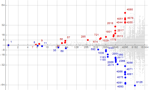
Among the high-water marks or records in c(n), we can find differences c(n) − n that themselves set records and record their indices in a superior sequence r. The first terms of the superior sequence r:
1, 7, 9, 45, 56, 57, 285, 674, 721, 1029, 1778, 1801, 2013, 2017, 2018, 4044, 4051, 4055, 4078, 4080, ...
Likewise, in the sequence u, we can find differences n − a(n) that set records and record their indices in an inferior sequence s. The first terms of the inferior sequence s:
1, 8, 11, 35, 60, 592, 1030, 1033, 1183, 1188, 2051, 2060, 2066, 2071, 2074, 2368, 4056, 4066, 4071, 4075, 4081, 4091, 4093, 8126, ...
Figure C2 generally plots c(n) in gray for 1 ≤ n ≤ 1000, but shows h(n) in dark red, and u(n) in dark blue. Zeroes in c(n) − n are marked in black. Recordsetters r in c(n) − n appear in large red points, some labeled. Minima in n − c(n) appear marked by large blue dots, also some of these are labeled.

Because the plot generally follows the slope 1, we might achieve a deeper analysis by running a log 10 plot of c(n) − n instead of c(n), as the values are never very far apart.
Figure C3 is a plot (x, y) = (n, c(n) − n), with 1 ≤ n ≤ 214, using a logarithmic scale on x.

This plot seems to show a balanced deviation from the line of slope 1. There seem to be repeated spikes associated with the motion of the previous value out of interval I( j) and into I( j + 1). Since c(n) is not far from n, the fractal behavior of the binary weight function w(n) is made evident, telegraphing through the the repeated pattern in its spikes, as the conditions that lead to one spike are present again as n transits the interval.
Figure C4 is the same logarithmic plot as Figure C3, but indicates the superiors r in red, many labeled, and the inferiors s in blue, also many labeled.
Records in c(n) are very common and make little sense to show in the log plot of c(n). The appearance of this plot resembles that for the function d(n) − n.
One of the conspicuous features evident in the plots of c(n) − n is the “flanging” or balanced spiking as the interval I( j) culminates, and at certain moments within the interval that seem to resemble the fractal sawtooth nature of the logarithmic plot of w(n) = A120. The function c(n) is never far from n (at least for small values of j), breaking out episodically to a new plateau. Because of the constraint of novelty of m, there are differences and warbles in the spikes so they do not exactly resemble similar structures that they seem to reflect in general configuration.
The effect of the value of w on c(n).
Figure C5 is a plot of w(n) for 1 ≤ n ≤ 1024 with the x-axis logarithmic, showing the least value of k = 1 in the interval I( j) = 2 j ≤ n ≤ (2( j + 1) − 1) with a large red dot, and the greatest value k = j + 1 with a large dot chromatically distant from red. We use the same color approach in Figures C6A and C6B. This plot demonstrates the “sawtooth” appearance of the function, favoring small k prevalent in the first half of the interval, and large k in the latter half. The fractal nature is better visible in Figure 1.

Figure C6A is a plot of c(n) − n for 1 ≤ n ≤ 4096, with the color function indicating the binary weight of the previous term c(n − 1) as in Figure C5, demonstrating that the spiking of c(n) seems somewhat registered with the behavior of w(n). Some of the early terms are easily picked out and we see the jumbling of certain features. See an enlarged plot of c(n) − n for 1 ≤ n ≤ 16384 with the same color function.

Figure C6B is a plot of c(n) − n for 212 ≤ n ≤ 214, showing the spikes or flanges in greater detail, demonstrating their rough self-similarity and regular spacing. We see c(n) with small w predominating the first half of the range in a pattern somewhat akin to the plot of w(n) in interval I(j).

These plots seem to suggest that w influences the amplitude and spacing of the spikes or flanges. When w is large, c(n) tends to respond with greater amplitude.
The effect of the binary weight function w(n) to c(n) is perhaps somewhat analogous to the effect of the digital root function via the exhaustion of digits available in the interval Ib( j) (in base b) of the previous term on d(n), in that the “flanging” or balanced spiking of the plot is instigated by features brought about by these functions.
Figure C7 is a log plot of c(n) for 1 ≤ n ≤ 212, showing even c(n) in red and odd c(n) in blue. See an image plotting only even or only odd values in c(n). The plot shows a slight bias for even numbers to be greater than the line with slope 1, and for odd numbers to fall below the same line.

There doesn’t seem to be much of a parity pattern beyond even m having a slight tendency to enter the sequence early.
Runs of the difference D = c(n) − n.
The function c(n) − n reveals runs of zeros whose length measures in the dozens at times. There are runs of other D that have length measuring 2, 3, or 4, which might be unremarkable otherwise.
Table C1 shows the least indices n such that there is a run length ℓ of consecutive differences D = c(n) − n, for 0 ≤ n ≤ 214. The first column is the run length ℓ, followed by the first position in c(n) where we start a zero difference. The column Q shows the number of instances of the run length ℓ of zeros in D. The column n that follows lists the first instance of a run length ℓ of D ≠ 0, with the final column showing the difference D.
L n Q n D
---------------------------
1 7
2 40 94 9 +2
3 210 12 32 +1
4 152 24 130 -2
5 122 41 403 -4
6 1 26 354 -1
7 13 31 434 -2
8 98 21 8897 -1
9 251 21 10125 -2
10 218 12
11 441 25
.
13 2293 4
14 468 4
15 4465 6
16 5233 2
17 971 2
18 2093 5
19 300 6
20 8235 1
21 827 1
22 3718 1
23 697 1
...
31 733 1
32 360 1
33 923 2
Therefore, we see that, beginning with c(923) = 923, we have 33 consecutive terms that are equivalent to their indices — and this happens twice, repeated at c(7435).
c(923) → 11100110112, binary weight w = 7 → 1112,
c(924) → 11100111002, w = 6 → 1102,
c(925) → 11100111012, w = 7 → 1112,
c(926) → 11100111102, w = 7 → 1112,
c(927) → 11100111112, w = 8 → 10002,
c(928) → 11101000002, w = 4 → 1002,
c(929) → 11101000012, w = 5 → 1012, ...
It is evident that these moments in c(n) occur when there exists a variety of patterns in n, once we have c(n) = n in interval I( j) with j = ⌊log2 n⌋, that sustain a range of most common w given I( j), that it is a chance alignment that is likely to repeat and perhaps sustain for longer runs.
Could we reach a point where D = 0 sustains infinitely? Consider the case of c(n) = j and thus c(n) = 2( j + 1) − 1 in interval I( j). We have w = j, yet the binary weight of 2( j + 1) is 1, thus unless j is a perfect power of 2, we will not have a pattern in the bits of 2( j + 1) to support w. Thus, at some point, any very long run of D = 0 must break.
Location in the binary expansion of k where w is found.
We may write a decimal analogy d(n) = A340138(n) to c(n), or for that matter, one in any base b > 2. If the decimal analogy replaces the binary weight w with the digital root d of the previous term, we observe that the early entrants to the sequence tend to find d among the very least significant digits. Does this tendency extend to finding w among the least significant bits of c(n)?
The principal difference between c(n) and d(n) aside from base is that d(n) concerns a single-digit digital root, while c(n) is concerned with binary weight that, if taken recursively to the fixed point, would prove to be 1 for all nonzero preceding terms. Therefore c(n) is perhaps more connected to a digital sum version of d(n) rather than to d(n) itself. Setting this aside, we see that, for d(n), we find d in one or more single-digit locations rather than concerning a range of bits signifying w written in binary at one or more locations in the binary expansion of some novel number m. Thus, we speak of finding w in initial (most significant) bits, medial bits, or final (least significant) bits of m. Additionally, we may find w throught m, as in the case of w = 1 in a number m that is a binary repunit (i.e., 2 j − 1. We may find w in initial and medial, or medial and final places, or in initial and medial places in m.
Figure C8 is a plot of c(n) − n for 1 ≤ n ≤ 214, showing the position in c(n) where w is found. Red signifies w found only in the most significant digits, blue the least significant bits of c(n). The enlarged plot accentuates the instances of w found in the most significant bits (red) and least significant bits (blue) by enlarging their dots, but w found in the most and least appear in magenta, w found in the most and medial in orange, least and medial in green, simply medial in gold, however the points are small and these are not as visible. This plot shows all points in medium size. This plot accentuates those points found in initial or final bits in the same red and blue respectively, but instead shows initial-and-medial in pink, medial-and-final in light blue, and both in light violet, letting medial finds remain small and gold.

This plot seems to illustrate that there is little connection between the behavior of the function and the location or locations in the binary expansion of c(n) where we find w. Any effect of the location in c(n) where we find w on the general nature of c(n) appears much less forceful than the somewhat analogous effect of d upon d(n), at least for 1 ≤ n ≤ 214.
In order to classify the positions where we find w in c(n), we use a three-bit number, with the first bit signifying w found in the most significant bits, the second with w in the medial position, and the third with w in the least significant position. Since we might find w in multiple places in the binary expansion of c(n), it is possible to occupy many of these at once. Therefore, we have 8 possible positions (including 0 meaning w is not found in c(n), which only applies to c(1) = 1).
000 0 No position.
001 1 Only in the most significant bits.
010 2 Only in medial bits.
011 3 In the most significant and medial bits.
100 4 Only in the least significant bits.
101 5 In both most and least significant bits, but not medial.
110 6 In the least significant and medial bits.
111 7 In all positions throughout.
The classification is imperfect; for “medial” bits, we do not distinguish extent; however in this scheme we are merely examining the presence of w in the least or most significant positions of c(n), whether associated with other locations or not.
Table C2 lists the number of positions of each kind in each interval I(j) = 2 j ≤ n ≤ (2( j + 1) − 1), with “+” signifying c(n) ≥ n, and “−” signifying c(n) < n.
most medial most & least most& least& w in all
only only medial only least medial positions
j + 1 - + 2 - + 3 - + 4 - + 5 - + 6 - + 7 -
----------------------------------------------------------------------------------
0 0 0 0 0 0 0 0 0 0 0 0 0 0 0
1 1 0 0 0 0 0 0 0 0 0 0 0 1 0
2 2 0 0 0 0 0 1 0 1 0 0 0 0 0
3 1 1 1 0 1 0 1 0 0 1 0 0 1 1
4 5 0 2 0 1 2 1 1 3 0 1 0 0 0
5 5 2 7 4 2 1 4 0 1 3 1 1 0 1
6 6 3 20 6 1 3 9 3 2 4 3 3 0 1
7 9 6 42 11 9 15 12 1 2 6 7 6 1 1
8 18 14 83 37 23 19 23 3 11 5 12 8 0 0
9 29 19 191 62 37 52 43 7 14 11 28 18 0 1
10 34 45 362 184 38 124 82 24 17 30 42 41 0 1
11 54 81 756 413 45 218 162 66 23 58 88 83 0 1
12 80 181 1515 1009 48 367 324 108 27 95 181 160 0 1
13 133 399 2948 2399 69 584 672 164 30 156 302 335 0 1
This data shows that there are some patterns in position of w in c(n), such as most and medial position (3) usually having c(n) found late, least-only (4) and medial-only (2) positions of w normally found early.
We list here the occasions of n for which w is found throughout the binary expansion of c(n):
n c(n) w c(n)_2 w_2
-------------------------------------
3 3 1 11 1
8 7 1 111 1
15 15 3 1111 11
35 31 3 11111 11
68 63 3 111111 11
128 127 3 1111111 11
255 255 7 11111111 111
515 511 3 111111111 11
1033 1023 3 1111111111 11
2074 2047 3 11111111111 11
4124 4095 3 111111111111 11
8202 8191 3 1111111111111 11
These happen to be repunits. The technical definition of the pattern (7) requires w in all places, however we might also see w = 2 found in c(12) = 10 in the most and least significant positions, i.e., “10” in “1010”. Of course we do not see “10” in the central position, but we might say that “10” covers “1010” back to back, accounting for all the bits in c(12). This case is left out of case (7).
Runs of the same value of w → c(n).
For the decimal digital root sequence d(n), we observed the run lengths of the same digital root d. Here we are instead interested in repeated applications of the same binary weight w.
We define sequence ℓ(n) by the number of consecutive binary weights of the same value w. If w is a singleton, it is assigned 1, but if it is duplicated, both are assigned 2, and part of a trio, 3 (given 16,384 terms of a(n), the largest run is 7).
Obviously, the occasion of repeated invocations of w stems from repeatedly obtaining the same binary weight across a range of c(n). Therefore we see that such repetitions only occur seven times in a row at most for a(n) with n ≤ 16,384.
The sequence ℓ(n) begins as follows (See Code 3.0):
2, 2, 1, 1, 2, 2, 1, 2, 2, 3, 3, 3, 2, 2, 1, 1, 2, 2, 2, 2, 1, 1, 1, 1, 2, 2, 1, 1, 1, 1, 1, 2, 2, 1, 1, 2, 2, 1, 2, 2, 1, 1, 1, 1, 1, 1, 1, 1, 1, 2, 2, 1, 1, 3, 3, 3, 1, 1, 1, 1, ...
Remember that ℓ(n) is not the list of run lengths, but rather, a mapping of the run-length to which w(c(n)) belongs; we are attempting to ascertain n for which w is repeated. Therefore, for 11 ≤ n ≤ 13 we have w = 2, so ℓ(n) = 3 in that range.
Table C3 tallies the number of singletons, doublets, triplets, etc. that occur in interval I( j) = 2 j ≤ n ≤ (2( j + 1) − 1).
j 1 2 3 4 5 6
------------------------------------
0 . 1/2 . . . .
1 1 1/2 . . . .
2 2 1 . . . .
3 1 2 1 . . .
4 10 3 . . . .
5 20 9/2 1 . . .
6 34 17/2 3 1 . .
7 72 22 4 . . .
8 133 50 5 2 . .
9 285 95 11 1 . .
10 598 153 36 3 . .
11 1291 243 79 7 . 1
12 2558 464 181 14 1 1
13 5090 929 385 17 3 1
Regarding c(n), we do not observe the sort of association we see in d(n), that repeated instigations tend to associate with amplitude. This said, we see some of the same features in one interval I( j) repeat and scale in the succeeding interval I( j + 1).
Figure C9 is a log plot of c(n) − n showing the degree of repetition of w that instigates m for 1 ≤ n ≤ 4096. Singletons are plotted tiny and gray, doublets in small dark blue, triplets in large cyan, quartets in green, quintets in gold, and sextets in large red (click here for an extended and enlarged plot for 1 ≤ n ≤ 16384):

Focusing on the intervals I(12) and I(13), we see similar repetition patterns in the spikes of the plot of c(n) − n.
Figure C10 is a log plot of c(n) − n showing the degree of repetition of w that instigates m for 4096 ≤ n ≤ 16384.

Depiction of terms of c(n) as a bitmap.
Figure C11 depicts c(n) in binary, with black = 1 and white = 0, starting with c(1) = 1 at left, vertically, the least bit at bottom, running through c(256) = 256 → 100000002 at right.
![]()
Figure C12 depicts c(n) in binary, with black = 1 and white = 0, starting with c(1) = 1 at left, vertically, the least bit at bottom, running through c(1024) = 1019 → 11111110112 at right.
![]()
The bitmaps seem to show that c(n) differs from the natural numbers mostly near the flipping of the most significant bits, shuffling the appearance of numbers in a tight zone there. It seems that c(n) is only slightly scrambled from the series of natural numbers. This is likely on account of c(n) having the most liberal conditions of the three sequences considered in this work.
Conclusion:
A sequence akin to this one in decimal, but pertaining to decimal digital roots, is explained in another paper, there called the “root-any” sequence, also known as the “frayed rope” sequence.
The sequence is a permutation of the natural numbers.
The sequence c(n) exhibits more complex behavior than a(n) or b(n), yet seems to hew close to c(n) = n. Where a(n) responds to congruency of w and m, separating into streams where the most common w in the interval I( j) conspire to press a given stream to set records, and b(n) responds to classes in each interval with a predictable cardinality, c(n) only varies a little from a line of slope 1 struck from the origin. The deviation appears to be governed mostly by the magnitude (perhaps as to log) of w.
Grand Conclusion.
We have examined three functions that find the bits of the binary weight of the previous term w somewhere in the binary expansion of a least novel current term m. The three sequences are different permutations of the integers since n appears at or before index 2n − 1, the first number with binary weight n.
The first “word→least” sequence a(n) finds w in the least significant bits of least novel m. This sequence features dendritic streams associated with a given word w that split at certain points, with the recordsetter streams changing according to the binomial frequency of w in interval I( j).
The second “word→most” sequence b(n) finds w in the most significant bits of least novel m. This sequence plot is characterized by the function jumping between streak-like “clouds” that represent classes according to the prefix w. Once the number of ( j + 1)- bit numbers that begin with w are exhausted, b(n) finds the prefix in the next interval.
Finally, the “word→any” sequence c(n) finds w in the most significant bits of least novel m. This sequence has a plot that varies only slightly from c(n) = n. The deviation of c(n) from n increases as the intervals culminate, seemingly as to the number of bits in w.
This concludes our exploration of the functions beginning with the first term 1 that use the binary weight of the previous term to determine the least novel m that serves as a new term.
Acknowledgements.
Special thanks to Michael S. Branicky and the editors of the OEIS.
Appendix:
Code A: Generate a(n) and store it in variable a:
a = Nest[Append[#,
Block[{k = 1, r = DigitCount[#[[-1]], 2, 1], s}, s = IntegerLength[r, 2];
While[Nand[FreeQ[#, k], Mod[k, 2^s] == r], k++]; k]] & @@ {#, Length@ #} &, {1}, 2^16];
Alternate approach using bits:
a = Nest[Append[#,
Block[{k = 1, r = IntegerDigits[DigitCount[#[[-1]], 2, 1], 2]},
While[Nand[FreeQ[#, k],
Take[IntegerDigits[k, 2], -Length@ r] == r], k++]; k]] & @@
{#, Length@ #} &, {1}, 2^8];
Code A1: Plot a(n) per Figure A1:
ListPlot[a[[1 ;; 2^12]], ImageSize -> Large, AspectRatio -> 1,
GridLines -> Automatic, PlotStyle -> {Blue, PointSize[Small]}] ]
Code A2: Plot a(n) per Figure A2:
With[{s = a[[1 ;; 2^8]], k = 2^3, j = 0},
ListPlot[MapIndexed[
Style[Labeled[#2, #2], Hue[(Mod[#2, k] + j)/k]] & @@ {#1, #2, #3,
If[# > 4, 2^(Floor[Log2@ #]) + Range[3]*2^(Floor[Log2@ #] - 2), {}] &[
2^Floor[#3]]} & @@
{First[#2], #1, Log2@ #1} &, s],
ImageSize -> Large, AspectRatio -> 1, PlotStyle -> PointSize[Large],
AspectRatio -> Automatic,
GridLines -> {2^Range[0, Ceiling@ Log2@ Length@ s],
2^Range[0, Ceiling@ Log2@ Length@ s]},
Ticks -> {2^Range[0, Ceiling@ Log2@ Length@ s],
2^Range[0, Ceiling@ Log2@ Length@ s]}] ]
Code A3: Plot a(n) per Figure A3:
With[{s = a[[1 ;; 2^12]], k = 2^3, j = 0},
ListPlot[MapIndexed[Style[#2, Hue[(Mod[#2, k] + j)/k]] & @@
{#1, #2, #3, If[# > 4, 2^(Floor[Log2@ #]) + Range[3]*2^(Floor[Log2@ #] - 2), {}] &[
2^Floor[#3]]} & @@
{First[#2], #1, Log2@ #1} &, s],
ImageSize -> Large, AspectRatio -> 1, PlotStyle -> PointSize[Small],
AspectRatio -> Automatic,
GridLines -> {2^Range[0, Ceiling@ Log2@ Length@ s],
2^Range[0, 1 + Ceiling@ Log2@ Length@ s]},
Ticks -> {2^Range[0, Ceiling@ Log2@ Length@ s],
2^Range[0, 1 + Ceiling@ Log2@ Length@ s]}] ]
Code B: Generate b(n) and store it in variable b:
b = Nest[Append[#,
Block[{k = 1, r = IntegerDigits[DigitCount[#[[-1]], 2, 1], 2]},
While[Nand[FreeQ[#, k], Take[IntegerDigits[k, 2], Length@ r] == r], k++]; k]] & @@
{#, Length@ #} &, {1}, 2^12]
Code B1: Plot b(n) per Figure B1:
ListPlot[b[[1 ;; 3*10^3]], ImageSize -> Large, ScalingFunctions -> "Log10",
GridLines -> Automatic, PlotStyle -> {Blue, PointSize[Small]}]
Code B2: Plot b(n) per Figure B2:
With[{s = wb[[1 ;; 2^7]]},
ListPlot[MapIndexed[
Style[Labeled[#2, ToString[#1] <> "." <> ToString[#2]],
Which[IntegerQ@ #3, Red, MemberQ[#4, #2], Hue[1/9], OddQ@ #2, Black, True, Hue[5/9]]] & @@
{#1, #2, #3, If[# > 4, 2^(Floor[Log2@ #]) + Range[3]*2^(Floor[Log2@ #] - 2), {}] &[
2^Floor[#3]]} & @@ {First[#2], #1, Log2@ #1} &, s],
ImageSize -> Large, AspectRatio -> 1, PlotStyle -> PointSize[Large],
AspectRatio -> Automatic,
GridLines -> {2^Range[0, Ceiling@ Log2@ Length@ s],
2^Range[0, Ceiling@ Log2@ Length@ s]},
Ticks -> {2^Range[0, Ceiling@ Log2@ Length@ s],
2^Range[0, Ceiling@ Log2@ Length@ s]}] ]
Code B3: Plot b(n) per Figure B4 (storing b(n) in variable wb):
Block[{lo = 2^3, hi = 2^8, j = 1, k = 9, wbf},
wbf = {1, 2, 4, 8, 16, 24, 32, 40, 48, 64, 80, 96, 128, 160, 192, 224,
256, 320, 384, 448, 512, 640, 768, 896, 1024, 1152, 1280, 1536,
1792, 2048, 2304, 2560, 2816, 3072, 3584, 4096, 4608, 5120, 5632,
6144, 7168, 8192, 9216, 10240, 11264, 12288, 13312, 14336, 16384,
18432, 20480} (* families *);
ListPlot[MapIndexed[Which[#1 < lo, ,
MemberQ[wbf, #2],
Style[Labeled[#2, #2, LabelStyle -> Bold], PointSize@ Large, Hue[(#4 - j)/k]],
True, Style[Labeled[#2, #4, LabelStyle -> Gray], PointSize@ Medium,
Hue[(#4 - j)/k]] ] & @@
{#1, #2, #3, If[#1 == 1, 0, DigitCount[wb[[#1 - 1]], 2, 1]]} & @@
{First[#2], #1, Log2@ #1} &, wb[[1 ;; hi]]],
ImageSize -> Large, PlotStyle -> PointSize[Tiny],
AspectRatio -> Automatic, PlotRange -> {{lo, hi}, {lo, 4 hi/3}},
ScalingFunctions -> {"Log2", "Log2"},
GridLines -> {2^Range[0, Ceiling@ Log2@ hi],
2^Range[0, Ceiling@ Log2@ hi]},
Ticks -> {2^Range[0, Ceiling@ Log2@ hi],
2^Range[0, Ceiling@ Log2@ hi]}] ]
Code B4: Plot b(n)/2v = b(n)/A7814(b(n)) with 1 ≤ n ≤ 256 per Figure B5 (storing b(n) in variable wb):
Block[{s, nn = 2^8, c = -1, d = 12, wbf, wbi, size = 24},
s = wb[[1 ;; nn]];
wbf = {1, 2, 4, 8, 16, 24, 32, 40, 48, 64, 80, 96, 128, 160, 192, 224,
256, 320, 384, 448, 512, 640, 768, 896, 1024, 1152, 1280, 1536,
1792, 2048, 2304, 2560, 2816, 3072, 3584, 4096, 4608, 5120, 5632,
6144, 7168, 8192, 9216, 10240, 11264, 12288, 13312, 14336, 16384,
18432, 20480} (* families *);
wbi = Map[Function[k, LengthWhile[wbf, # <= k &] ], wb] (* Family Indexing *);
Show[{ListPlot[
MapIndexed[
If[Or[IntegerQ@ #3, MemberQ[#4, #2]],
Style[Labeled[#6, StringJoin[ToString[#1], ".", ToString[#2]]],
PointSize@ Large, Hue[(#7 + c)/d]],
Style[Labeled[#6, FromDigits@ IntegerDigits[#7, 2],
LabelStyle -> Gray],
PointSize@ Which[IntegerQ@ #3, Large, MemberQ[#4, #2], Large,
OddQ@ #2, Medium, True, Medium], Hue[(#7 + c)/d]]] & @@
{#1, #2, #3, Which[
#1 >= 8192, 2^(Floor[Log2@ #1]) + {1, 2, 3, 4, 5, 6, 8}*2^(Floor[Log2@ #] - 3),
#1 >= 2048, 2^(Floor[Log2@ #1]) + {1, 2, 3, 4, 6, 8}*2^(Floor[Log2@ #] - 3),
#1 >= 1024, 2^(Floor[Log2@ #1]) + {1, 2, 4, 6, 8}*2^(Floor[Log2@ #] - 3),
#1 >= 128, 2^(Floor[Log2@ #1]) + Range[3]*2^(Floor[Log2@ #] - 2),
#1 >= 32, 2^(Floor[Log2@ #1]) + {1, 2, 4}*2^(Floor[Log2@ #] - 2),
#1 >= 16, 2^(Floor[Log2@ #1]) + Range[3]*2^(Floor[Log2@ #] - 1),
#1 >= 2, 2^(Floor[Log2@ #1]) + 2^(Floor[Log2@ #] - 1),
True, {}] &[2^Floor[#3]], wbi[[#1]], #2/2^Floor[#3],
If[#1 == 1, 1, DigitCount[wb[[#1 - 1]], 2, 1]]} & @@ {First[#2], #1, Log2@ #1} &, s],
ImageSize -> 900, ScalingFunctions -> {"Log2", Automatic}, AspectRatio -> 1,
PlotStyle -> PointSize[Tiny],
GridLines -> {2^Range[0, Ceiling@ Log2@ nn], 1 + Range[0, #]/# &@ 8},
Ticks -> {2^Range[0, Ceiling@ Log2@ nn],
2^Range[0, Ceiling@ Log2@ nn]}],
Graphics[{LightGray,
Style[Text["1000", {.5, 1.0625}], FontSize -> size],
Style[Text["1001", {.5, 1.1875}], FontSize -> size],
Style[Text["1010", {.5, 1.3125}], FontSize -> size],
Style[Text["1011", {.5, 1.4375}], FontSize -> size],
Style[Text["1100", {.5, 1.5625}], FontSize -> size],
Style[Text["1101", {.5, 1.6875}], FontSize -> size],
Style[Text["1110", {.5, 1.8125}], FontSize -> size],
Style[Text["1111", {.5, 1.9375}], FontSize -> size]}]} ] ]
Code C: Generate c(n) and store it in variable c:
c = Nest[Append[#,
Block[{k = 1, r = IntegerDigits[DigitCount[#[[-1]], 2, 1], 2]},
While[Nand[FreeQ[#, k], SequenceCount[IntegerDigits[k, 2], r] > 0], k++]; k]] & @@
{#, Length@ #} &, {1}, 2^12]
Code C1: Plot c(n) per Figure C1:
ListPlot[c[[1 ;; 2^12]], ImageSize -> Full, AspectRatio -> 1,
GridLines -> Automatic, PlotStyle -> Directive[Blue, PointSize[Small] ] ] ]
Code C2: Plot c(n) similar to Figure C2:
ListPlot[MapIndexed[#1 - First[#2] &, c],
ImageSize -> Large, PlotRange -> {All, {-72, 72}},
ScalingFunctions -> {"Log10", Automatic}, GridLines -> Automatic,
PlotStyle -> PointSize[Small]]
Concerns OEIS sequences:
A000120 Binary or Hamming weight of n; number of 1s in the binary expansion of n.
A007318 Pascal’s Triangle, or the triangle T(n,k) = binomial(n, k).
A007814 2-adic valuation of n; number of trailing zeros in the binary expansion of n.
A049773 Triangular array T read by rows: if row n is r1, …,rm, then row n + 1 is 2r1 − 1, …,2rm − 1,2r1, …,2rm.
A248025 Lexicographically earliest permutation of the positive integers such that the first digit of a(n+1) is the digital root of a(n).
A338191 a(1) = 1, a(n) is the least m not already in a(n) such that m mod 10 = decimal digital root of a(n − 1).
A338209 a(n), the “word → least” sequence.
A339024 b(n), the “word → most” sequence.
A339607 c(n), the “word → any” sequence.
A340138 d(1) = 1, d(n) is the least m not already in d(n) such that the decimal digital root of d(n − 1), is found anywhere within the decimal expansion of m, a decimal analogy to c(n).
Document Revision Record.
2020 1016 2300 First draft.
2020 1129 2030 Second draft.
2020 1219 2200 Publication of Sequences.
2021 0122 0715 Publication of A340138.