Constitutive Analysis of the EKG Sequence

(OEIS A064413 by Jonathan Ayres, 2001 0930.)

Written by Michael Thomas De Vlieger, St. Louis, Missouri, 2021 1130-1208.

Abstract.

The EKG sequence is a permutation of the natural numbers that has a simple recursive functional definition that prohibits equality and coprimality of adjacent terms j and k. Hence primes are forced into divisorship and because of this, they appear late in the sequence. As a consequence, the sequence exhibits Lagarias-Rains-Sloane or LRS chains 2p→p→3p. Another consequence is that most k belong to the cototient of j such that j and k each have at least 1 prime factor q that does not divide the other (i.e., j and k are mutually semicoprime). We examine 3 quasi-linear striations QLS in the log-log scatterplot and number-theoretical relationships between j and k. There are 6 constitutive binary relationships seen in the sequence, and 2 key signatures associated with primes and prime powers that are not prime. A juxtaposition of these signatures pertains to Fermat primes in the sequence. We summarize certain terms that represent landmarks in the EKG sequence in the Appendix.

Introduction.

Let us examine the sequence defined as a(n) = n for n ≤ 2; for n > 2, a(n) = least distinct k such that gcd(j, k) > 1, where j = a(n−1). The first terms are:

1, 2, 4, 6, 3, 9, 12, 8, 10, 5, 15, 18, 14, 7, 21, 24, 16, 20, 22, 11, 33, 27, 30, 25, 35, 28, 26, 13, 39, 36, 32, 34, 17, 51, 42, 38, 19, 57, 45, 40, 44, 46, 23, 69, 48, 50, 52, 54, 56, 49, 63, 60, 55, 65, 70, 58, 29, 87, 66, 62, 31, 93, 72, 64, 68, 74, 37, 111, 75, 78, 76, 80, 82, 41, 123, 81, 84, 77, 88, 86, 43, 129, 90, 85, 95, 100, 92, 94, 47, 141, 96, 98, 91, 104, 102, 99, 105, 108, 106, 53, 159, 114, 110, 112, 116, 118, 59, 177, 117, 120, 115, 125, 130, 122, 61, 183, 126, 119, 133, 140, ...

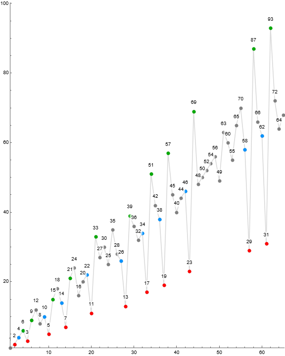
This sequence is known as the “EKG” or ectocardiogram sequence for the appearance of its scalar scatterplot at small scale when points are joined by lines, as in Figure 1. We have generated 300000 terms of a through Code 1, later over 10 million via Code 4. The smaller dataset is the basis of observations described in this work unless noted otherwise.

The sequence a begins with seed terms {1, 2}, where the first term is a “dead seed” that does not affect the recurrent mappings of the sequence function. Perceivably, 1 appears so as to render a a permutation of the natural numbers. It is understandable that the effective seed 2 is selected, for 1 would fail to generate a result, and seed m > 2 would eventually find k = 2 given any even instigator. Then the recursive mappings of the sequence function would proceed as usual until m and any odd terms that follow it interfere with forbidden equality.

The sequence mandates a “bridging factor” 1 < gcd(j, k) = A073734(n − 1).

Figure 1: Scatterplot of a(n) for 1 ≤ n ≤ 64, showing primes p in red, 2p in blue, and 3p in green.

Recognizing the occasion of 3 prominent quasi-linear striations (QLS) in a log-log scatterplot, we arrange terms k in a in 4 groups [1, 2]:

The first 18 terms comprise an agglomeration δ of juxtaposed number types not clearly in any QLS.
Central γ if k is neither p prime nor 3p, then k/n ≈ n.
Upper α if k = 3p, then k/n ≈ 3n/2.
Lower β if k = p, then k/n ≈ n/2.

The sequence scatterplot is simple, with 2 of 3 QLS easy to explain. The central γ is a catch-all melange of several kinds of numbers. Constitutive properties of QLS are described in a section below.

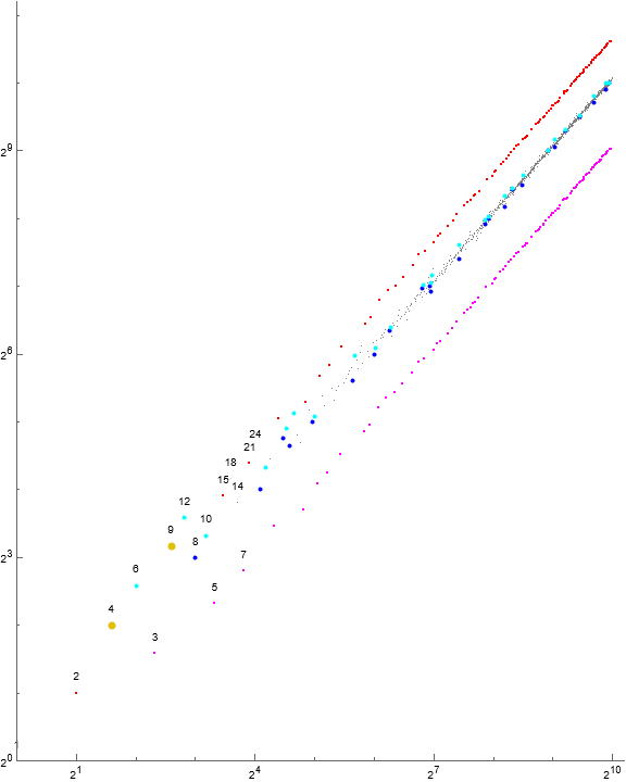
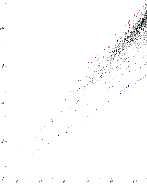
Figure 2: Log-log scatterplot of a(n) for 1 ≤ n ≤ 2¹⁰, showing primes p in red corresponding completely to QLS β, 2p in blue corresponding to central γ along with other terms, and 3p in green, corresponding completely to QLS α. The first 12 terms of the sequence do not clearly respect the QLS, hence form an agglomeration δ. Use Code 2 to plot this figure.

Theorems from other papers and approach of this paper.

This sequence has been extensively studied [2, 3] and we have the fortune of some useful theorems:

The sequence a is a permutation of the natural numbers.
Primes p = a(n) occur in increasing order as n increases.
For odd p, we have the chain 2p → p → 3p.
Conception of a instead via “controlling primes”, which we shall describe later.

Theorem 3 supports observed striations; we find 3p in α, p in β, and 2p along with other k in central γ. We term the chain mentioned in Theorem 3 the “LRS chain”.

The approach in this work is to examine a in terms of recursive mappings of a function f( j) → k, where the function f is defined as:

{f( j) → k : j ∧ k ∈ N, k ∉ a(1..n−1), (j, k) > 1},
starting with seed {1, 2},
where 1 has no effect on the sequence.

Hence, this work is not as concerned with slopes as are [2, 3], save as a general observation, as the mappings do not heed the index n except reference to that part of a already generated by the remappings.

Since the recursive mappings of f do not rely on n except to ensure distinct k, it is not surprising that the fixed points A064420 in a are finite.

This paper examines the sequence via constitutive relations between j and k. Some reminders are shown here for easy reference. (Links in this paper refer to points in the constitutive relations paper where a full explanation of terms appears. Further, we have used the nomenclature of [4] in speaking of constitutive relations for concision. We have done this in order to keep this paper brief.)

Table 1.1 summarizes the constitutive binary relations and their qualities. Examples appear in the note. For coprimality, we may consider any 2 dissimilar primes p and q. Symmetrical divisibility applies only to j = k, which is forbidden.

C	\|	binary relation	abb.	sym.	neut.	reg.	rev.	note
----	\|	------------------	------	------	------	------	------	----------------
⓪	\|	j ⊥ k ∧ k ⊥ j	⊥	✓			⓪	∀ p, q, p ≠ q
①	\|	j ◊ k ∧ k ◊ j	◊.◊	✓	✓		①	6, 10
②	\|	j ◊ k ∧ k \| j	◊.\|				④	30, 6
③	\|	j ◊ k ∧ k \|\| j	◊.\|\|		✓		⑦	30, 12
④	\|	j \| k ∧ k ◊ j	\|.◊				②	10, 30
⑤	\|	j \| k ∧ k \| j	\|.\|	✓		✓	⑤	∴j = k
⑥	\|	j \| k ∧ k \|\| j	\|.\|\|			✓	⑧	6, 12
⑦	\|	j \|\| k ∧ k ◊\| j	\|\|.◊		✓		③	20, 30
⑧	\|	j \|\| k ∧ k \| j	\|\|.\|			✓	⑥	20, 10
⑨	\|	j \|\| k ∧ k \|\| j	\|\|.\|\|	✓	✓	✓	⑨	12, 18

Table 1.2: General constitutive outline of A064413. The state is listed at left, followed by the index n of first instance j ◯ k, the cardinality in the dataset, cardinality of parity associated with the state, and cardinality of prime j and k.

Constitutive census of A064413 (EKG Sequence, 10^7 terms)
      First instance               Parity             Primality
State  n    j    k     card.       2|j       2|k      p_j      p_k
------------------------------------------------------------------
(0)    1    1    2         1         0         1        0        1
(1)   11   15   18   9288228   4749555   5105311        0        0
(2)    4    6    3    355314    355314         0        0   355314
(3)    7   12    8       579       525        29        0        0
(4)   10    5   15    355313         0         0   355313        0
(6)    2    2    4         2         1         1        2        0
(7)    3    4    6       563        24        77        0        0

Some facts regarding the outline above, based on 10 million terms:

State ⓪ is a technicality, since 1 ⊥ 2, which is forbidden by sequence definition, though 1 and 2 are seed (given) terms.
Completely regular state ⑥ is the rarest. It pertains to 2→4 and 3→9 early in the sequence.
We do not expect to see further instances of state ⑥, which is an artifact of early terms.
The mixed neutral states ③ and its reverse, ⑦ are somewhat rare.
1. State ③ is the input state of prime powers that are not prime (except for the above-mentioned 2 instances of state ⑥).
2. Singleton state ③ pertains additionally to 20 other numbers that are defects from state ①. Here is a list of the first 6:
  a(1220) = 1290 → 1280, gcd = 10
  a(5845) = 6105 → 6075, gcd = 15
  a(45635) = 47306 → 47089, gcd = 217
  a(47290) = 48894 → 48878, gcd = 58
  a(65225) = 67396 → 67228, gcd = 28
  a(245686) = 252770 → 252448, gcd = 322
  We expect further defects that become more rare as n increases.
3. State ⑦ is the output state of prime powers that are not prime.
4. We find singleton state ⑦ in 2 additional cases:
  a(1383878) = 1417176 → 1417182, gcd = 6
  a(4381471) = 4478976 → 4478982, gcd = 6
Divisor states ② and its reverse, ④ are not as rare and pertain to primes.
1. State ② is the input state of prime k, since k | j therefore j > k.
  This state interposes 2p ◊.| p in the LRS chain.
  This state therefore exits QLS α for QLS β.
  There is a single defect that introduces prime 2, that is 1 ⓪ 2
2. State ④ is the output state of prime j, since j | k therefore j < k.
  This state interposes p |.◊ 3p in the LRS chain.
  This state thus exits QLS β to join central γ.
  There are 2 defects associated with 2 ⑥ 4 and 3 ⑥ 9.
The ambidirectional, completely neutral, symmetrically semicoprime state ① predominates the sequence. It represents chaos and comprises the lion’s share of QLS central γ.
States ⑧ and ⑨ are not prohibited but do not appear.
1. State ⑧ is the reverse of state ⑥ and would come about via p^ε → p^(ε−i), i ≥ 1 and other rare relations. We do not anticipate p^ε → p^(ε−i), i ≥ 1, since the prime powers that are not prime in a appear in central γ hence in order of magnitude. We do not anticipate this state.
2. State ⑨ is a generally rare state that requires rad(j) = rad(k) for j and k both composite. The state pertains to numbers that are within the same regular space, such being relatively sparse compared to the coprime and semicoprime spaces, if the state hadn’t appeared when n is small, it is exponentially unlikely to appear as n increases, since there are always smaller unused k not confined to regular space .We do not anticipate this state.

The EKG sequence has a decent degree of order since 4 of the 5 observed states and their reversals (if applicable) present in the sequence can be linked to a specific kind of term in the sequence. Two states that do not appear are not anticipated. See the Appendix Table A for terms that are landmarks in the EKG sequence.

Figure 3: Log-log scatterplot of a(n) for 1 ≤ n ≤ 2¹⁰, color-coded to show constitutive states that generate k = a(n). Tiny gray dots have state ①, medium-sized dark blue ③, medium-sized cyan ⑦, comprising central γ. Magenta dots correspond to p and state ② in QLS β. Red dots correspond to 3p and state ④ in QLS α. Large gold dots pertain to state ⑥. State ⓪ that “generates” k = 2 shows red in this plot.

Consequences of definition.

Consequences of the definition of a are that coprimality and equality of j and k are not allowed, hence we do not have states ⓪ or ⑤ in a. Because we are looking for least k, the sequence a has a least unused number u (the smallest missing number in the sequence a(i) for 1 ≤ i < n). This partitions the potential k into three segments:

The unsaturated segment k > r. We say herein that such k is “unused” or “unplayed”.
The semisaturated segment u ≤ k ≤ r.
The saturated segment 1 ≤ k < u. We say herein that such k is “played” or “used”.

We can write a sequence u(i) = A152458(i) for 1 ≤ i < n for that contains the least unused number as we generate a. It is interesting to take the distinct terms in u; we end up with the primes in order according to Theorem 2.

Conception of the EKG sequence via “controlling primes”.

Lagarias-Rains-Sloane [2] wrote an algorithm (see Code 4) that approaches the EKG sequence in a different manner than the recursive-functional definition we have discussed, or the original definition of the sequence.

LRS conceived of a counter akin to the least-unused seeker function u(n) applied to many recursive mapping sequences requiring distinct terms k.

Suppose we have a sequence s(n) beginning with 1 that is a remapping of f( j) → k : least k ∉ s(1…n−1). This sequence thus features a least unused number u_n (Sloane calls a smallest missing number or SMN). The function may eventually encounter input j = u_n. When this happens, we use a while statement to iterate u until we find a new least-unused number u_(n+1), since there are oftentimes “sticky“ SMN that, whereupon entering the sequence, we have a new local minimum bound. This u is a discrete lower bound for s. For a, the discrete lower bound is the sequence A8578, that is the sequence of 1 and the primes. Hence, in A064413 sequence, given input j = u_n, function u( j) sets u_(n+1) = nextprime( j), a prudent shortcut given a is a permutation of the natural numbers.

The LRS algorithm requires memoization of A020639, i.e., the sequence of the least prime factors or lpf(n), as this would be required as a reference via their function “small(n)” instead of refactorization of n to find same. At same time, we generate a sequence quot(n) = n/lpf(n) = A032742(n), the largest proper divisor d | n. Furthermore, the LRS algorithm employs registers c(p) : p prime, that find the least missing mp : m > 0 ∧ p prime. Whereupon we have k in a, we update c(p) for all p | k.

The LRS algorithm achieves the following. Starting with the limit ℓ which is the largest number k we desire to find (not the number of terms we wish to generate) we set m = ℓ. We whittle m down via conditional recursion upon k = min(k, c(lpf(j))) ∧ m = quot(m) until m = 1. Once we have k by this means, we update c(p) for all p | k. Hence we have the concept of a governing factor or “controlling prime” p for each k. The paper showed that p | (j, k). The paper also mentions that more than one controlling prime (hence, governing factor) applies to k.

Hence the sequence function instead is something like this:

Let registers c(p) = jp : j > 0 ∧ p prime ∧ jp ∉ a(1…n−1).

Therefore set k = min(k, c(A020639( j))) while recursively reducing m via A032742(m) until reaching a fixed point, followed by updating c(p) for all p | k thereafter.

Seen this way, we understand why examining the occurrence of mp in a behaves the way it does. Furthermore, A064413 becomes a matter of the least controlling prime on j, i.e., A064740( j), and appropriately selecting k = c(p). This alternate definition of the sequence certainly is more complicated to express than the original or official definition. See Code 4.1 for a rendition of LRS code that generally matches variables in this paper.

Parity and rough numbers.

Even composites j have a relatively dense set of potential k, since gcd(j, k) > 2 implies k belonging to the cototient of j. The cototient of even j comprises at least half of the range {1…( j − 1)}, hence there are more options k < j, and more frequent options k > j, especially if j is highly divisible.

In the 300000-term EKG sequence dataset, it is more than 50% more likely that j > k for j even, indicating that even j finds k in the cototient. Furthermore, the average move, | k − j |, is small; there are 36618 instances of k = j + 2, 15497 instances of k = j + 4, 5967 of k = j − 4, and 5398 instances of k = j − 2. Most of the large moves are negative: of the 14684 distinct differences k − j for j even, only 12 of them are positive and the largest is +16.

Table 2.1: directionality of R-rough j.

        | k - j |
R    dec.     inc.    total
----------------------------
2   93965    60095   154060
3   39734   106204   145938
5    9606    80619    90225
7    4900    64785    69685
11    2877    55070    57947
13    1832    49613    51445
17    1372    45247    46619
19    1001    42141    43142
...

Given the recursive mapping of the function f in sequence a, it is clear k belongs to the cototient of j. We see that even j affords the highest cototient density, (j − φ(j))/j ≥ ½. Therefore, we should expect j > k more often, as well as minimal | k − j | for even j as opposed to odd j, 5-rough j, 7-rough j, etc., where an R-rough number m has least prime factor lpf(m) ≥ R prime. An R-rough number is less likely to result in k < j as R increases, since the cototient grows more rarified as R increases.

Table 2.2: Constitutive analysis of input states for even, odd, 5-rough, …, R-rough numbers in a.

Input (j)                 R-Rough
State     2       3       5      7     11     13
------------------------------------------------
(0)       1       -       -      -      -      -
(1)  153993  117307   75852  55334  43609  37216
(2)       -   14190   14189  14188  14187  14186
(3)      20     140     130    124    118    114
(4)       -   14190       -      -      -      -
(6)       1       1       -      -      -      -
(7)      45     111      54     39     33     29

Table 2.3: Constitutive analysis of output states for even, odd, 5-rough, …, R-rough numbers in a.

Output (k)                R-Rough
State     2       3       5      7     11     13
------------------------------------------------
(1)  139718  131583   75891  55362  43632  37237
(2)   14190       -       -      -      -      -
(3)     134      78      16     12     10      8
(4)       -   14190   14189  14188  14187  14186
(6)       1       1       -      -      -      -
(7)      17     139     129    123    118    114

Even j instigates state ① most often. The case of even squarefree semiprimes is a subset of even j instigating state ②, i.e., 2p ◊.| p. Indeed, we have 2p → p in state ②, but also, for example, j = 50 → 52, j = 54 → 56 . The sole case of even j instigating state is 2 ⑥ 4. Completely neutral states ③ and ⑦ are rare defects of state ①. Where we normally have state ① ◊.◊, we at times have ◊.|| or ||.◊, which correspond to states ③ and ⑦, respectively.

Prime powers that are not prime.

Generally in this work, we write “prime powers” exclusive of primes themselves, i.e., numbers in A246547.

Perfect powers 2^ε = a(n) for n in A064954. The progenitor j → 2^ε must also be even since ω(2^ε) = 1 and gcd( j, k) > 2. The difference | 2^ε − j | ≤ 12 in the dataset, showing that even j “creeps into” 2^ε for k near n. Hence, 2^ε occurs “as a matter of course” along with other even numbers, but results from j ◊.|| 2^ε outside of the defects of the given {1, 2} and 2 |.|| 4. The only way we could have j | 2^ε is if j < 2^ε is also a perfect power of 2, and that only occurs at 2 |.|| 4, hence state ⑥. The completely regular states are increasingly unlikely, as 2^ε < k necessarily lies in the unsaturated segment and there are many smaller even k, thus we do not see adjacent 2^ε except for 2 → 4. We are left with state ③.

Table 3.1: Analysis of a(n) = 2^ε for 1 ≤ ε ≤ 23, showing progenitor j and difference k − j.

      n        j  State      k  k-j
-----------------------------------
      2        1  (0)        2    1
      3        2  (6)        4    2
      8       12  (3)        8   -4
     17       24  (3)       16   -8
     31       36  (3)       32   -4
     64       72  (3)       64   -8
    122      124  (3)      128    4
    240      258  (3)      256   -2
    485      522  (3)      512  -10
    982     1030  (3)     1024   -6
   1961     2044  (3)     2048    4
   3932     4094  (3)     4096    2
   7898     8196  (3)     8192   -4
  15820    16386  (3)    16384   -2
  31729    32764  (3)    32768    4
  63576    65548  (3)    65536  -12
127354   131076  (3)   131072   -4
255162   262146  (3)   262144   -2
511014   524354  (3)   524288  -66
1023398  1048578  (3)  1048576   -2
2049132  2097148  (3)  2097152    4
4102601  4194298  (3)  4194304    6
8213244  8388622  (3)  8388608  -14
...

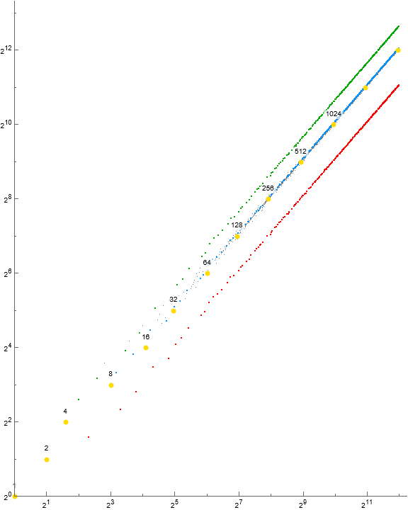
Figure 4: Log-log scatterplot of a(n) for 1 ≤ n ≤ 2¹², superimposing the powers of 2 in gold upon Figure 2.

Suppose we have a prime power p^ε : ε > 1. This number p^ε is unlike most composites since it has 1 distinct prime factor p, i.e., ω(p^ε) = 1.

Therefore p^ε-regular numbers are starkly bifurcated such that p^(ε−i) < p^ε : 0 < i ≤ ε are divisors, and p^(ε+i) > p^ε are semidivisors. We see 2 instances of adjacent p |.|| p^ε in 2→4 and 3→9, which is constitutive state ⑥ between them. Otherwise, prime powers p^ε : ε > 1 appear after 3p in the sequence not adjacent to p, since p² lies in the unsaturated segment at least until we have k = 3p, the least novel k in the cototient of p, i.e., k ≡ 0 (mod p). Indeed there are many multiples mp : m < p that must enter the sequence before p² owing to its magnitude [2]. In fact, in the dataset, we see p(p+1)→p² : p ≠ q, q ∈ {2, 3, 157, 661, …}, the first case outside of 2 and 3 at a(23831) = 158×157, a(24146) = 157². This attributes to the action of controlling primes described in [2].

Generally p^ε : ε > 1 appears amid mp in vicinity via neutral relation, since there is always k < p^(ε+1) belonging to the cototient of j : p | j, and p^ε finds k < p^(ε+1) such that belongs to the k-cototient. The adjacency of prime powers p^ε : ε > 1 ∧ p > 3 is impossible on account of the geometric progression on p, because there is always a smaller k that satisfies function f.

Hence we have .|| p^ε ||. as powers of the same prime, outside of 2→4 and 3→9, are nonadjacent due to the way they are instigated. This restricts input states to j ③ p^ε ∨ j ⑥ p^ε, the latter iff j = p^ε−i, i ≥ 1, and consequently j < p^ε. Output states are restricted to p^ε ⑦ k. Generally, prime powers p^ε : ε > 1 relates to composite m : ω(m) > 1 ∧ p | m in the mode p^ε ||.◊ m , hence states ③ or ⑦. Such may only relate to p^{(ε + i)} : e > 1 ∧ | i | ≥ 1, that is, adjacent prime powers divisible by the same prime, via mode p^ε ||.| p^{(ε + i)}, hence states ⑥ or ⑧. The last-mentioned state is not seen since prime powers that are not prime appear in order of magnitude in a.

Given a dataset of 10954981 terms, there are 581 instances of p^ε : ε > 1. Of these, there are 44 cases of j < p^ε and 537 to the contrary. Both cases 2 |.|| 4 and 3 |.|| 9 represent j < p^ε; the remaining 42 cases have nondivisor j : ω( j) > 1 in the cototient of p^ε. In all 581 cases, p^ε < k, as a consequence of p^ε ||.◊ k, since nondivisor k regular to p^ε must exceed p^ε.

Table 3.2: Constitutive signatures associated with prime powers p^ε : ε > 1. The power appears between the first and second states in the signature. Generally the prime pattern is ② p ④, while the prime-power pattern is ③ p^ε ⑦. There are various defects from the general pattern for both primes and prime powers.

ε\p 2 3 5 7 11 13 17 19
----------------------------------
1 067 267 241 241 243 241 241 241
2 672 673 371 371 371 371 371 371
3 372 373 ... ... ... ... ... ...
4 371 371
5 372 ...
6 371
7 373
8 371
9 372
10 371
11 ...

The general signature for prime powers k = p^ε in a is “371”, that is, pm ◊.|| p^ε ||.◊ pm' ◊.◊. For prime p, the pattern is “24(1∨3)”, that is, pm ◊.| p |.◊ pm' ◊.◊ or pm ◊.| p |.◊ pm' ◊.||. We will explain the defects in 2^ε and 3.

There are 2 instances of prime powers in a separated by 1 term, which has signature “373”. The first is 3³ → 30 → 5², hence has signature “373”, that is, 33 ◊.|| 27 ||.◊ 30 ◊.|| 25. The second is 2⁷ → 132 → 11², hence has signature “373”, that is, 124 ◊.|| 128 ||.◊ 132 ◊.|| 121.

In a, we find that states ③ and ⑦ typically signify the input and output modes, respectively, of prime powers p^ε that are not prime. There are certain defects that induce other states, i.e., input state ⑥ iff preceded by p^a : 1 ≤ a < ε, and output state ⑥ iff followed by p^a : a > ε.

Primes.

Prime k | j as a consequence of forbidden coprimality, hence prime k is confined to states ② or ⑧ which imply sequence decrease. Furthermore, the reverse situation, prime j | k, i.e., the term that follows primes in a is confined to states ④ or ⑥ which imply increase.

The LRS chain.

Let’s examine the LRS chain 2p → p → 3p. Odd primes p in the sequence arise from even squarefree semiprimes 2p and generate 3p, since 2p preceded p and is not available. Since p | k, we must have k (mod p) ≡0, therefore k = mp, integer m > 1, hence, we iterate on m and thus consider 2p, 3p, 4p, etc. in turn, but per Theorem 3, 2p has always been played, and it is never necessary to seek beyond 3p, since it is always available.

Why does 2p induce p? Recall that p is restricted to the divisible states; 2p ◊.| p for p > 2 (otherwise, 4 ||.| 2, which is not seen since 2 is given!) and p |.◊ 3p for p > 3 (otherwise 3 |.|| 9). Hence, some composite j instigates prime k.

Since the sequence has the “least k” constraint, even semiprimes 2p are the least multiple mp to enter the sequence for p > 2. These induce p since there is no method except for divisibility to bring them in.

In a we find that states ② and ④ typically signify the input and output modes, respectively, of prime p. One significant defect has output state ⑥ iff followed by p^ε : ε > 1, cf. 2→4 and 3→9. We see p = 2 has forbidden input state ⓪ since {1, 2} are (given) seeds.

Constitutive analysis of the LRS chain.

Generally, for prime p > 3, we have 2p ◊.| p |.◊ 3p, which means that p divides both the previous and the following terms, but understandably, both 2p and 3p are multiples mp where m ⊥ p. We may express this in terms of states as 2p ② p ④ 3p, and diagrammatically as the following:

2p → p → 3p
(①) → ② → ④

We therefore read the constitutive signature “(1)24” as at least some of the time pertaining to the occasion of prime k. We do not always observe the penultimate term (the term before 2p) exhibiting state ①.

Note the “bridging factors” that are the least prime divisors common to j ∧ k for the initiator and the successor to the LRS chain:

j : 2 | j → 2p → p → 3p → k : 3 | k

This is a consequence of the limitations on squarefree semiprimes with the smallest least prime factors. The small factors appear most often in the cototient of j or k. In the case of the successor to 3p, we would otherwise have 4p, as in the case of 3→9→12 where it was still accessible. For larger primes, the next multiple of 3 is smaller. As a consequence, for i > 1, A073734(A064955(i) − 1) = 2 and A073734(A064955(i) + 2) = 3.

The first prime k = 2 is an exception to the chain 2p → p → 3p as 2 is given, but interpreting it constitutively, we see that we have the forbidden relation 1 ⊥ 2. Since 2p = 2(2) = 4 has not appeared, we have 2 |.|| 4, hence 2 ⑥ 4. This chain, rendered in terms of constitutive relations, becomes:

1 → 2 → 4
◯ → ⓪ → ⑥

where the first relation, ◯, represents a given term. The appearance of state ⑥ is perchance, since p |.|| 2p implies even prime p. For odd p, the relation requires state ④, p |.◊ 2p.

We look to the occasion of the next prime, 3, for something resembling the general case. We have the following regarding p = 3:

4 → 6 → 3 → 9
⑦ → ② → ⑥

Relationally, this is 4 ||.◊ 6 ◊.| 3 |.|| 9. The appearance of state ⑥ here is also perchance, since p |.|| 3p implies trine prime p. For nontrine odd primes p (i.e., all p > 3), we have state ④, since p |.◊ 3p.

Constitutive signatures associated with Fermat primes.

What is interesting about the signature “726” for prime p = 3 is the introduction to the chain via state ⑦. Obviously, we have this state because introducing term 4 ||.◊ 6.

Let the chain for primes like 3 be such:

J → 2p → p → 3p,

Suppose we do not know the introducing term J, but of course the first term in the LRS chain, 2p, is even. Since we know 2 | 2p and via Theorem 3, it is clear p has not appeared. Hence Theorem 3 implies p ⊥ J, J is constrained to states ①, ④, or ⑦.

Since 2p is a squarefree semiprime, we may only have state ④ iff J = 2 or J = p; we know the latter is not possible. We have already seen 2 in the sequence; it generated the term 4 and thus we never see J ④ 2p with p odd. We therefore are left with 2 cases: signature “124” or “724” for odd primes p. We note that state ⑦ presents only two possibilities: 2^ε ||.◊ 2p and p^ε ||.◊ 2p. The latter is prohibited since mp remains in the unsaturated segment k > r by the “least k” constraint, and along with it, p^ε.

The case of constitutive signature “724” may only occur for J = 2^ε, ε > 1, since any other even J presents some other prime factor q ⊥ p, seeing all mp in the unsaturated segment k > r.

The sequence A064954(ε) lists indices n such that a(n) = 2^ε. The powers of 2 appear in order at least for 0 ≤ ε ≤ 24.

The signature “724” associates with Fermat primes {3, 5, 17, 257, 65537} = A019434. This Fermat-LRS chain has the following structure for p > 3:

j : 2 | j → 2^ε → 2p → p → 3p → k : 3 | k
③→⑦→②→④→①
where 2p = 2^ε+ 2 and p = 2^(ε−1)+1.

Hence we see that in Table 3.2 the “372” signature pertaining to 2^ε associates with Fermat primes.

Table 4.1: A list of the terms that surround a(n) = p such that p is a Fermat prime. The constitutive binary relation (state) between the terms appears parenthetically below each list.

a(5)           2        4        6       3        9       12        8
         (0)      (6)      (7)      (2)      (6)      (7)      (3)

a(10)         12        8       10       5       15       18       14
         (7)      (3)      (7)      (2)      (4)      (1)      (1)

a(33)         36       32       34      17       51       42       38
         (1)      (3)      (7)      (2)      (4)      (1)      (1)

a(487)       522      512      514     257      771      513      516
         (1)      (3)      (7)      (2)      (4)      (1)      (1)

a(131076) 131076   131072   131074   65537   196611   131079   131085
         (1)      (3)      (7)      (2)      (4)      (1)      (1)

Constitutive signatures.

The EKG sequence is a fairly simple sequence in terms of constitutive signatures.

Let c(n) be the sequence of states that a(n) generates. This sequence begins as follows, generated by Code 2:

0, 6, 7, 2, 6, 7, 3, 7, 2, 4, 1, 1, 2, 4, 1, 3, 7, 1, 2, 4, 3, 7, 3, 7, 1, 1, 2, 4, 1, 3, 7, 2, 4, 1, 1, 2, 4, 1, 1, 1, 1, 2, 4, 1, 1, 1, 1, 1, 3, 7, 1, 1, 1, 1, 1, 2, 4, 1, 1, 2, 4, 1, 3, 7, 1, 2, 4, 1, 1, 1, 1, 1, 2, 4, 3, 7, 1, 1, 1, 2, 4, 1, 1, 1, 1, 1, 1, 2, 4, 1, 1, 1, 1, 1, 1, 1, 1, 1, 2, 4, 1, 1, 1, 1, 1, 2, 4, 1, 1, 1, 3, 7, 1, 2, 4, 1, 1, 1, 1, 1, ...

Completely neutral, symmetrically semicoprime state ① generally comprises the sequence outside of certain special cases. Completely neutral binary relations require j and k both composite, sharing at least 1 prime factor between them, but not all, and not all distinct prime factors. Most often, the bridging factor is the least prime factor common to both j and k, since it presents the most open cototient.

Given the dataset of 10 million terms, there are 20 occasions where j ◊.|| k, thus isolated state ③, rather than j ◊.◊ k and mixed neutral state ①. These defects appear to be happenstance. There is no reason to rule out more isolated state ③ instances as n increases. Likewise, there are 2 occasions of j ||.◊ k, thus singleton state ⑦. Therefore, singleton mixed-neutral states appear 22 times in 10 million terms of a. (See Appendix Table B.)

Generally, the signature ②④ pertains to primes, while ③⑦ pertains to prime powers p^ε : ε > 1.

The few defects from these general patterns are easily demonstrated and explained in their respective sections [primes], [prime powers]. We summarize these here:

1 ⓪ 2 ⑥ 4, instead of ②④, since 1 is given, and 2 |.|| 4 (adjacent p and p^ε : ε > 1).
2 ⑥ 4 ⑦ 6, instead of ③⑦, since 2 |.|| 4 (adjacent p and p^ε : ε > 1).
6 ② 3 ⑥ 9, instead of ②④, since 3 |.|| 9 (adjacent p and p^ε : ε > 1).
3 ⑥ 9 ⑦ 12, instead of ③⑦, since 3 |.|| 9 (adjacent p and p^ε : ε > 1).

These essentially constitute collisions of the signatures on account of juxtaposition of primes and their powers.

Table 5.1: constitutive signatures in the first 10954981 terms of the EKG sequence, ignoring state ①. See Codes 2 and 5.

signature      card.       n   first instance of signature
--------------------------------------------------------------------------
         3        20     1220   {1290 (3) 1280}
         7         2  1383878   {1417176 (7) 1417182}
        24    386691       13   {14 (2) 7 (4) 21}
        37       567       16   {24 (3) 16 (7) 20}
      2437         4       73   {82 (2) 41 (4) 123 (3) 81 (7) 84}
      3724         3       31   {36 (3) 32 (7) 34 (2) 17 (4) 51}
      3737         1      120   {124 (3) 128 (7) 132 (3) 121 (7) 143}
    243737         1       19   {22 (2) 11 (4) 33 (3) 27 (7) 30 (3) 25 (7) 35}
0672673724         1        1   {1, 2, 4, 6, 3, 9, 12, 8, 10, 5, 15}

There are several agglomerations of the signatures that are seen only once, and a couple thrice:

The collisions described above occur at the start of the sequence, involving its first 11 terms. This leads to an agglomeration of the states ⓪⑥⑦②⑥⑦③⑦②④. This run and the immediately following term a(12) = 18 comprise agglomeration δ.
There is a run of primes and powers intercalated with composites beginning at a(19): 22 ② 11 ④ 33 ③ 27 ⑦ 30 ③ 25 ⑦ 35.
There is a further instance of prime powers separated by 1 composite beginning at a(120): 124 ③ 128 ⑦ 132 ③ 121 ⑦ 143.
There are 3 instances of a prime power and a prime, separated by 1 composite; these pertain to the Fermat primes {32, 34, 17}, {512, 514, 257}, {131072, 131074, 65537} (see Table 4.1). If we include the instance of ③⑦②④ that pertains to 5, then this is the general signature of Fermat primes p > 3.
There are 4 instances of a prime and a prime power separated by 1 composite:
1. 82 ② 41 ④ 123 ③ 81 ⑦ 84,
2. 2182 ② 1091 ④ 3273 ③ 2187 ⑦ 2190,
3. 19678 ② 9839 ④ 29517 ③ 19683 ⑦ 19692.
4. 531434 ② 265717 ④ 797151 ③ 531441 ⑦ 531444

It is unknown whether the condition observed in the fourth case strictly concerns instances of Fermat primes, but certainly corresponds to the known ones. Outside of this case, all but the fifth case above do not seem to present a chance to repeat.

A summary of constitutive landmarks in the EKG sequence appears in the Appendix Table A.

Constitutive properties of striations.

The most conspicuous feature of the so-called EKG sequence’s scatterplot seen in aggregate (Figures 2 and 3) are the α, central γ, and β quasi-linear striations (QLS). The α appears above and β below the central γ QLS. The agglomeration of data in the first 18 terms called δ is simply where the jitter of the QLS intermingles early on in the sequence. Yet we may refine the definition of α instead as containing k = 3p : prime p > 3, and β as containing (odd) prime k. Central γ consists of what is left over.

Beta Striation. The indices of prime p = k in the EKG sequence, specifically, in QLS β, comprise OEIS A064955. The ratio k/j = ½ inbound and 3 outbound, with exception for k = 2, where the inbound ratio is 2 and outbound is 2. We have the following input and output states; for p = 2, ⓪ 2 ⑥, p = 3, ② 3 ⑥, and generally, ② p ④. Prime p requires a divisor state, i.e., .| p |. since coprimality is forbidden. This is the reason for the reluctance of primes to enter the sequence, requiring a multiple mp : m = 2 for p > 2 to introduce them.

Alpha Striation. The indices of k in QLS α is tantamount to A064955(n) − 1 : n > 2. The successor to primes p in a appear in α QLS. Therefore, in terms of QLS, the LRS chain has this general relationship with quasi-linear striations in the scatterplot of the EKG sequence:

{j : 2|j} ① 2p ② p ④ 3p ① {k : 3|k}
γ ① γ ② β ④ α ① γ

Central Gamma Striation. In central γ, we have several states, but predominantly the QLS contains the completely neutral, symmetrically semicoprime j ① k, characterized by minimal | k − j |, with either parity, however k is slightly more likely than j to be even. In this state, j and k are composite with at least 2 distinct prime factors.

The singleton mixed neutral states ③ and ⑦ are rare defects that transpire when j ◊.|| k or more rarely, j ||.◊ k.

Central γ QLS contains prime powers p^ε : ε > 1, which, on account of ω(p^ε) = 1, are restricted to .|| p^ε ||., hence the signature ③⑦ (save in a couple cases already mentioned). State ③ introducing normally features j > p^ε. Both defects 2 ⑥ 4 ⑦ 6 and 3 ⑥ 9 ⑦ 12 have j < p^ε, since j | p^ε. We know that vis-à-vis p^ε : ε > 1, state ⑦ implies p^ε < k as a consequence of p^ε ||.◊ k, since nondivisor k regular to p^ε must exceed p^ε.

All 20 observed cases of singleton state ③ feature j > k : k is in the cototient of j, however j < k is not forbidden. Hence, γ₃ usually induces increase if ω(k) = 1, while the rare γ₆ always induces increase.

Both observed cases of singleton state ⑦ feature j > k : k is in the cototient of j, however j < k is not forbidden. Hence, γ₇ induces increase iff ω( j) = 1.

Constitutively restricted variations.

The definition of a prohibits coprimality and equality of j and k, that is, constitutive binary relations (states) ⓪ and ⑤, respectively. We now consider some additional restrictions on the function and what sort of sequence results.

Shannon’s Enots Wolley sequence (A336957) begins with {1, 2, 6}. Let i = A336957(n−2) and j = A336957(n−1). Then for n > 3, i ① k ∧ j ⓪ k. Ignoring {1, 2}, this sequence is essentially the EKG sequence limited to ①. Indeed, another of Shannon’s sequences, A337687, excepting the initial 2, is more directly the EKG sequence limited to ①.

Noting that the primes in a have signature ②④, what happens if we restrict k to divisor states, i.e., ②④⑥⑧? This is tantamount to sequence s_D that is the recursive mapping of f defined below:

{f( j) → k : j ∧ k ∈ N, k ∉ a(1..n−1), (j, k) = j ∨ k},
starting with seed {1, 2},
where 1 has no effect on the sequence.

Showing binary relations between terms, this sequence begins:

s_D = [1 ⓪ 2] ⑥ 4 ⑥ 8 ⑥ 16 ⑥ 32 ⑥ 64 ⑥ 128 ⑥ … = A79.

This is because we started with a seed p : ω(p) = 1. Let’s start with the least seed j : ω( j) > 1:

6 ⑧ 2 ⑥ 4 ⑥ 8 ⑥ 16 ⑥ 32 ⑥ 64 ⑥ 128 ⑥ …

Once we reach k : log₂ k ∈ N, we re-enter A27. We may choose any number j : ω( j) > 1, but the sequence will eventually merge into A27.

Consider the sequence s_SD generated by restriction of j ◯ k to states ② or ④, beginning with seed 2. Here we may only have either j | k ∧ k ◊ j its reverse, j ◊ k ∧ k | j. This sequence begins:

2, 6, 3, 12, 4, 20, 5, 10, 30, 15, 60, 420, 7, 14, 42, 21, 84, 28, 140, 35, 70, 210, 105, 630, 9, 18, 90, 45, 180, 36, 252, 63, 126, 1260, 315, 1890, 27, 54, 270, 135, 540, 108, 756, 189, 378, 3780, 945, 5670, 81, 162, 810, 405, 1620, 324, 2268, 567, 1134, 11340, 2835, 17010, 243, 486, 2430, 1215, 4860, 972, 6804, 1701, 3402, 34020, 8505, 51030, 729, 1458, 7290, 3645, 14580, 2916, 20412, 5103, ...

The sequence is not a permutation of the natural numbers, since after a(22) = 210, we enter a kind of recurrence of order 12; we see neither 11 nor 13 or any larger primes, and all numbers in the sequence are in A2473.

Seeing the special status of signatures ②④ and ③⑦ in a, we consider restriction to those states. These are semicoprime-divisor and mixed neutral states. This sequence, s20211205 = A353916, has seed 2 and begins as follows:

2, 6, 3, 12, 4, 10, 5, 15, 9, 18, 8, 14, 7, 21, 27, 24, 16, 20, 25, 30, 32, 22, 11, 33, 66, 36, 42, 28, 49, 35, 70, 40, 60, 45, 81, 39, 13, 26, 64, 34, 17, 51, 102, 48, 78, 52, 128, 38, 19, 57, 114, 54, 84, 56, 126, 63, 105, 75, 90, 50, 110, 44, 121, 55, 125, 65, 130, 80, 120, 72, 132, 88, 154, 77, 231, 99, 165, 135, 150, 96, 138, 23, 46, 230, 92, 256, 58, 29, 87, 174, 108, 156, 104, 169, 91, 182, 98, 140, 100, 170, 68, 204, 136, 238, 112, 168, 144, 180, 160, 190, 76, 228, 152, 266, 133, 343, 119, 289, 85, 255, ...

Figure 6.1: Log-log scatterplot of A353916(n), 1 ≤ n ≤ 256, labeling records in red, local minima in blue.

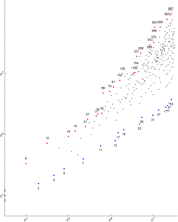
Prime powers appear in the records:

2, 6, 12, 15, 18, 21, 27, 30, 32, 33, 66, 70, 81, 102, 128, 130, 132, 154, 231, 256, 266, 343, 372, 465, 620, 625, 820, 940, 987, 1180, 1239, 1281, 1340, 1407, 1420, 1491, 1533, 1659, 2046, 2937, 3597, 3729, 4521, 4587, 4917, 5379, 5511, 5709, 5907, 5973, 6303, 6474, 6561, 6882, 8034, 8502, 8814, 9477, 10005, 11622, 12714, 13026, 13494, 13689, 14118, 15625, 19683, ...

The least unused u are primes as in a.

The constitutive states begin as follows:

4, 2, 4, 2, 7, 2, 4, 3, 4, 3, 7, 2, 4, 3, 7, 3, 7, 3, 7, 3, 7, 2, 4, 4, 3, 7, 3, 3, 7, 4, 3, 7, 3, 3, 7, 2, 4, 3, 7, 2, 4, 4, 3, 7, 3, 3, 7, 2, 4, 4, 3, 7, 3, 7, 2, 7, 3, 7, 3, 7, 3, 3, 7, 3, 7, 4, 3, 7, 3, 7, 3, 7, 2, 4, 3, 7, 3, 7, 3, 7, 2, 4, 4, 3, 3, 7, 2, 4, 4, 3, 7, 3, 3, 7, 4, 3, 7, 3, 7, 3, 4, 3, 7, 3, 7, 3, 7, 3, 7, 3, 4, 3, 7, 2, 3, 7, 3, 7, 4, 3, ...

Figure 6.2: Log-log scatterplot of A353916(n), 1 ≤ n ≤ 2¹², showing records in red, local minima in blue.

Sequence A353916 merits some exploration that lies beyond the scope of this paper.

Consider a sequence t = t20211127 = A240024 limited to states ①③⑦⑨, thus confined to composites, beginning with seed 4. This is tantamount to recursive mappings of the following function f defined as follows:

{f( j) → k : j ∧ k ∈ N, k ∉ a(1..n−1), 1 < (j, k) > min( j, k)},
starting with seed 4 and confined to composites.

The sequence t begins:

4, 6, 8, 10, 12, 9, 15, 18, 14, 16, 20, 22, 24, 21, 27, 30, 25, 35, 28, 26, 32, 34, 36, 33, 39, 42, 38, 40, 44, 46, 48, 45, 50, 52, 54, 51, 57, 60, 55, 65, 70, 49, 56, 58, 62, 64, 66, 63, 69, 72, 68, 74, 76, 78, 75, 80, 82, 84, 77, 88, 86, 90, 81, 87, 93, 96, 92, 94, 98, 91, 104, 100, 85, 95, 105, 99, 102, 106, 108, 110, 112, 114, 111, 117, 120, 115, 125, 130, 116, 118, 122, 124, 126, 119, 133, 140, 128, 132, 121, 143, 154, 134, 136, 138, 123, 129, 135, 141, 144, 142, 146, 148, 150, 145, 155, 160, 152, 156, 147, 153, ...

In actuality the sequence never plays state ⑨ for reasons related to the situation seen in a. The only signature outside of repeated ① and the singleton ⑦ associated with t(1) = 4 is ③⑦, pertaining to the occasion of p^ε : ε > 1 in t. The sequence t has a tight scatterplot and may be a permutation of the composite numbers. It merits exploration that lies beyond the scope of this work.

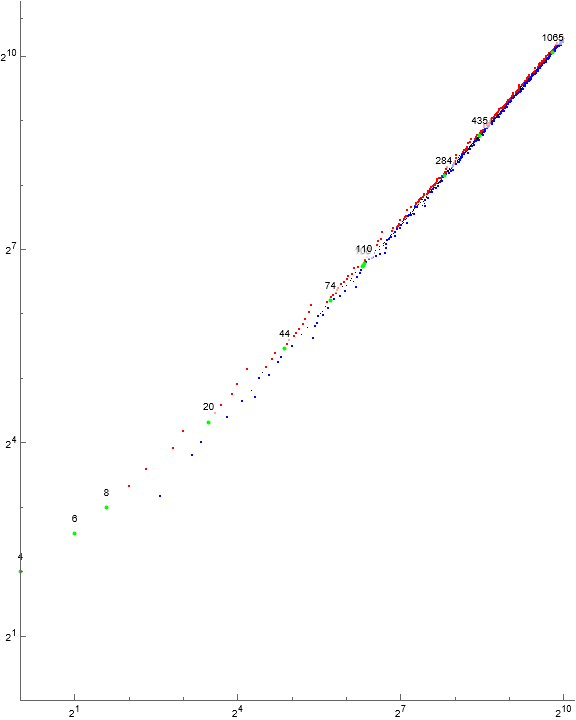
Figure 6.3: Log-log scatterplot of A240024(n), 1 ≤ n ≤ 64, labeling records in red, local minima in blue.

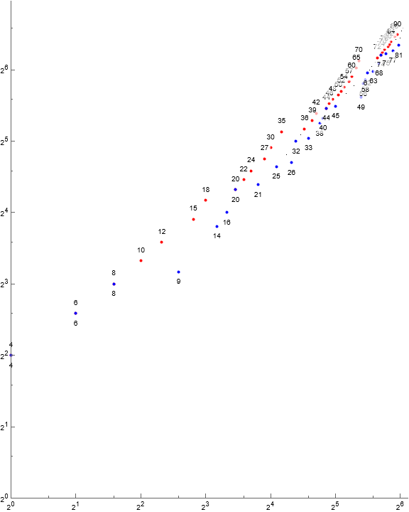
Figure 6.4: Log-log scatterplot of A240024(n), 1 ≤ n ≤ 2¹⁰, showing records in red, local minima in blue. Green, labeled terms are those that are records and local minima.

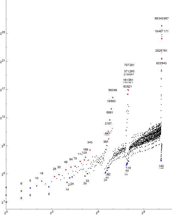
We finally consider a sequence v = t20211205 = A353917, limited to ③⑦ and thus composites, beginning with 4. The sequence is caustic, with Cunningham-like chains instead within j-regular numbers when prime powers emerge. The sequence plays semicoprimality against semidivisibility, the former favoring small moves while the latter commands moves at scale according to numbers regular to j akin to geometric progression. This sequence merits exploration that lies beyond the scope of this work.

The constitutive states of A353917 begin as follows:

7, 3, 7, 3, 7, 3, 7, 3, 7, 7, 3, 3, 7, 3, 7, 3, 7, 3, 7, 7, 3, 7, 3, 7, 3, 7, 3, 7, 3, 7, 3, 7, 3, 3, 7, 3, 7, 3, 7, 3, 7, 3, 7, 3, 7, 7, 3, 7, 3, 7, 3, 7, 3, 7, 3, 7, 3, 7, 3, 7, 3, 7, 3, 7, 3, 7, 3, 7, 3, 7, 3, 7, 3, 7, 3, 7, 3, 7, 3, 7, 3, 7, 3, 7, 3, 3, 7, 3, 7, 3, 7, 3, 7, 3, 7, 3, 7, 3, 7, 3, 7, 3, 7, 3, 7, 3, 7, 3, 7, 3, 7, 3, 7, 3, 7, 3, 7, 3, 7, 3, ...

Generally the states alternate, but not always. The first occasion of a run of state ⑦ appears at v(10) = 20 and concerns 25 ⑦ 20 ⑦ 30. The first occasion of a run of state ③ appears at v(12) concerning 30 ③ 18 ③ 27.

Figure 6.5: Log-log scatterplot of A353917(n), 1 ≤ n ≤ 360, showing records in red, local minima in blue. Green, labeled terms are those that are records and local minima.

In all the constitutively restricted variations on the EKG sequence, ironically, eliminating “disorder” of state ① only seems to have imparted chaos into scatterplot.

Conclusion.

In this paper we have examined the EKG sequence A064413 according to recursive mappings of a function f( j) → k, where the function f is defined as:

{f( j) → k : j ∧ k ∈ N, k ∉ a(1..n−1), (j, k) > 1},
starting with seed {1, 2},
where 1 has no effect on the sequence.

Consequently, coprimality and equality, corresponding to constitutive states ⓪ and ⑤, are prohibited.

Building upon previous papers and the Lagarias-Rains-Sloane chain 2p→p→3p, we used constitutive analysis in order to describe four principal features of the log-log scatterplot seen in Figure 2. The four features include 3 quasi-linear striations (QLS) α corresponding to 3p and constitutive state ②, β corresponding to prime p and constitutive state ④, and central γ containing the other states. An agglomeration δ kicks off the sequence, comprised of the first 12 terms that do not appear to heed QLS. This agglomeration begins with 11 contiguous constitutive states that are not state ①.

Examining the constitutive states c in the sequence, we identified general constitutive signatures before and after primes (②④) and prime powers not prime (③⑦). We identified defects from these states, including the only 2 instances of state ⑥ in the sequence, 20 cases of isolated state ③, 2 cases of singleton state ⑦, and juxtapositions of the prime and prime-power signatures. Notably, signature ③⑦②④ pertains to Fermat primes in a. The sequence otherwise is dominated by state ① in central γ. Two completely regular states ⑧ and ⑨ are not seen, though not prohibited by definition, but rather the mechanics of the sequence.

Finally, we took a look at a few interesting sequences that placed additional constitutive restrictions on the relationship between adjacent terms. Several merit study that lies beyond the scope of this work.

This concludes our examination.

Appendix

Table A: Landmarks in A064413.

The following are constitutive landmarks in the EKG sequence. They represent unique or first instances of patterns seen in the sequence, explained at the constitutive census and the constitutive signature segment of this work.

General landmarks:
a(1,2) = 1 ⓪ 2; given terms.
a(1..11) = {1,2,4,6,3,9,12,8,10,5,15} longest run of states ≠ ①.
a(1..18) = {1,2,4,6,3,9,12,8,10,5,15,18,14,7,21,24,16,20} δ group.
a(2,3) = 2 ⑥ 4, first instance of state ⑥.
a(4,5) = 3 ⑥ 9, last instance of state ⑥.
a(11,12) = 15 ① 18, first instance of state ①.
a(13..15) = 14 ② 7 ④ 21; first prime with standard signature ②④
a(16..18) = 24 ③ 16 ⑦ 20; first prime power with standard signature ③⑦
a(19..21) = {22,11,33} unambiguous beginning of α, central-γ, and β QLS, respectively.
a(19..25) = 22 ② 11 ④ 33 ③ 27 ⑦ 30 ③ 25 ⑦ 35, sole instance of ②④③⑦③⑦.
a(120..124) = 124 ③ 128 ⑦ 132 ③ 121 ⑦ 143, sole instance of conjoined ③⑦
a(1220..1221) = 1290 ③ 1280, first case of singleton state ③. (see Table B).
a(1383878..1383879) = 1417176 ⑦ 1417182, first case of singleton state ⑦. (see Table B).

Fermat prime signatures (generally) ③⑦②④:
a(2..6) = 2 ⑥ 4 ⑦ 6 ② 3 ⑥ 9
a(7..11) = 12 ③ 8 ⑦ 10 ② 5 ④ 15
a(30..34) = 36 ③ 32 ⑦ 34 ② 17 ④ 51
a(484..488) = 522 ③ 512 ⑦ 514 ② 257 ④ 771
a(127353..127357) = 131076 ③ 131072 ⑦ 131074 ② 65537 ④ 196611

near-adjacent prime-prime power signature ②④③⑦:
a(19..23) = 22 ② 11 ④ 33 ③ 27 ⑦ 30
a(73..77) = 82 ② 41 ④ 123 ③ 81 ⑦ 84
a(2093..2097) = 2182 ② 1091 ④ 3273 ③ 2187 ⑦ 2190
a(19030..19034) = 19678 ② 9839 ④ 29517 ③ 19683 ⑦ 19692
a(517979..517983) = 531434 ② 265717 ④ 797151 ③ 531441 ⑦ 531444

Table B: A list of singleton mixed neutral cases in a.

Singleton mixed neutral states
      n        j  State      k
------------------------------
   1220     1290  (3)     1280
   5845     6105  (3)     6075
  45635    47306  (3)    47089
  47290    48894  (3)    48778
  65225    67396  (3)    67228
245686   252770  (3)   252448
319075   327850  (3)   327680
342024   351260  (3)   351232
541053   555770  (3)   555025
1065864  1093070  (3)  1092025
1383878  1417176  (7)  1417182
1767175  1810370  (3)  1809025
2305772  2359302  (3)  2359296
2919285  2985978  (3)  2985984
3045828  3116990  (3)  3115225
3299709  3376406  (3)  3374569
4171146  4266290  (3)  4264225
4381471  4478976  (7)  4478982
5137793  5251743  (3)  5250987
5410762  5529832  (3)  5529503
7462741  7625882  (3)  7623121
8468838  8652422  (3)  8649481
...

References:

[1] N. J. A. Sloane, Seven Staggering Sequences, 2006, see p. 1-3.

[2] J. C. Lagarias, E. M. Rains, and N. J. A. Sloane, The EKG sequence, arXiv:math/0204011 [math.NT], 2002.

[3] Piotr Hofman and Marcin Pilipczuk, A few new facts about the EKG sequence, J. Int. Seq., 11 (2008), Article 08.4.2.

[4] Michael De Vlieger, Constitutive Relations, 2021.

Code 1: Generate a (generates 2¹² = 4096 terms in 3.5 s, 2¹⁴ = 16384 terms in 64 s). Code based on increment on k, with shortcuts based on proofs in [3]. Generates 2¹⁶ terms in 1200 s. Appears in [4]. Variable c akin to hit in Code 4; j = a(n−1), k = a(n) sought, s = given terms, u = least unused term (Dr. Neil Sloane calls such “SMN, smallest missing number”). Written 2021 1119.

Block[{c, j, k, s = {1, 2}, u = 3}, c[_] = 0;
  Set[j, 2]; Array[Set[c[#], #] &, 2];
  Range[2]~Join~Reap[Monitor[Do[
    If[PrimeQ[j], Set[u, NextPrime[j]]];
    Set[k, u];
    While[Nand[c[k] == 0, GCD[j, k] > 1], k++]; Sow[k];
    Set[c[k], i]; j = k, {i, 4, 2^12}], i]][[-1, -1]]]

Code 2: Produce constitutive states for terms in a. (Set the span notation as required)

Block[{s = Partition[a064413[[1 ;; 2^8]], 2, 1], a, b},
  a = Map[Which[Mod[#2, #1] == 0, 0,
    PowerMod[#2, #2, #1] == 0, 1, True, -1] & @@ # &, s];
  b = Map[Which[Mod[#1, #2] == 0, 0,
    PowerMod[#1, #1, #2] == 0, 1, True, -1] & @@ # &, s];
  {0}~Join~(1 + Rest@ Array[3*(1 + a[[#]]) + (1 + b[[#]]) &, Length[a]])]

Code 3: Plot Figure 2.

Block[{nn = 2^10, a, s, q, qq, out = -120},
  a = A064413[[1 ;; nn + 1]];
  Table[Set[s[i], Array[If[PrimeQ[#/i], #, out] &@ a[[#]] &, nn]], {i, 3}];
  ListPlot[
  Join[{a}, Array[s[#] &, 3], {Array[Labeled[#, #, Top] &@ a[[#]] &, 2^4]}],
    ImageSize -> Large, ScalingFunctions -> {"Log2", "Log2"},
    PlotRange -> {{1, nn}, {1, Max[a]}}, AspectRatio -> Full,
    PlotStyle -> {
      Directive[Gray, PointSize[Tiny]],
      Directive[Red, PointSize[Small]],
      Directive[Hue[4/7], PointSize[Small]],
      Directive[Darker[Green], PointSize[Small]],
      Transparent}]]

Code 4: Efficient generation of a via LRS code modeled on that in [2], page 4-5. Generates 1365159 terms in 90 s. Based on the phenomenon of “controlling primes” explained in [2]. Variable names largely match [1]. Variable b distinct from B so as to disambiguate during generation as we encounter a recursion error. Also, k = a(n−1). Otherwise, functions exactly as described in [2]. Note: the user-defined limit nn pertains to the largest value a(n) desired in the sequence, not the number of terms. Hence, nn = 2²¹ has the program run until it reaches a number that exceeds 2²¹. This program breaks at that point, drops the final term, and yields the dataset. “Decoded” from [2] 2021 1207 2130. May furnish over 10 million terms.

Block[{nn = 2^21, B, b, hit, gap, small, quot, p, k},
  B[_] = hit[_] = gap[_] = small[_] = quot[_] = 0;
  Set[k, 2]; Set[B[2], 2]; Array[Set[hit[#], 1] &, 2];
  Monitor[Do[
    Set[{small[i], quot[i]}, {#1[[1, 1]], Times @@ Power @@@ #2}] & @@
    TakeDrop[FactorInteger[i], 1], {i, 2 nn}], i];
  {1}~Join~Most@ Reap[Monitor[Do[If[k == nn, Break[], b = nn;
    While[k > 1, Set[p, small[k]]; Set[b, Min[b, B[p]]];
      Set[k, quot[k]]]; Sow[b]; Set[hit[b], 1];
    Map[If[B[#] == 0,
      Set[B[#], #], (Set[j, B[#]/#]; While[hit[# j] > 0, j++];
      Set[B[#], # j])] &, FactorInteger[b][[All, 1]]];
    k = b], {i, 3, nn}], i]][[-1, -1]]]

Code 4.1: Here is a version of Code 4 that connects with the section in this paper that discusses LRS controlling prime concept:

Block[{nn = 2^24, c, h, j, k, m, n, p, a020639, a032742},
  c[_] = h[_] = a020639[_] = a032742[_] = 0; m = j = c[2] = 2;
  Array[Set[h[#], 1] &, 2];
  Monitor[Do[
    Set[{a020639[i], a032742[i]}, {#1[[1, 1]], Times @@ Power @@@ #2}] & @@
      TakeDrop[FactorInteger[i], 1], {i, nn}], i];
  {1}~Join~Most@ Reap[Monitor[Do[
    If[m == nn, Break[], k = nn;
    While[m > 1, Set[p, a020639[m]]; Set[k, Min[k, c[p]]];
      Set[m, a032742[m]]]; Sow[k]; Set[h[k], 1];
    Map[If[c[#] == 0,
      Set[c[#], #], (Set[n, c[#]/#]; While[h[# n] > 0, n++];
      Set[c[#], # n])] &, FactorInteger[k][[All, 1]]];
    m = j = k], {i, 3, nn}], i]][[-1, -1]]]

Code 5: Generate a constitutive census of a similar to Table 5.1 (Store results from Code 1 or Code 4 in a064413, and store results from Code 2 in c064413).

Block[{nn = 2^16, s, t},
  s = a064413[[1 ;; nn + 1]];
  t = c064413[[1 ;; nn]];
  Map[{
    StringJoin["(", ToString[#1], ")"], #2, #3, #4,
    Count[t, #1],
    With[{k = #1},
      Count[Position[t, k][[All, 1]], _?(EvenQ@ s[[#]] &)]],
    With[{k = #1},
      Count[Position[t, k][[All, 1]], _?(EvenQ@ s[[# + 1]] &)]],
    With[{k = #1},
      Count[Position[t, k][[All, 1]], _?(PrimeQ@ s[[#]] &)]],
    With[{k = #1},
      Count[Position[t, k][[All, 1]], _?(PrimeQ@ s[[# + 1]] &)]]} & @@
  Flatten@ {#1, #2, s[[#2]], s[[#2 + 1]]} & @@
    {#, FirstPosition[t, #][[1]]} &, Union@ t]] // TableForm

Concerns sequences:

A000040: The primes.
A000079: 2ⁿ, n ≥ 0.
A002473: 7-smooth numbers.
A002808: The composite numbers.
A019434: Fermat primes {3, 5, 17, 257, 65537}.
A020639: Least prime factor of n, lpf(n).
A032742: n/lpf(n); greatest proper divisor d | n.
A064413: EKG sequence: a(n) = n for n ≤ 2; for n > 2, a(n) = least distinct k such that gcd(j, k) > 1, where j = a(n−1).
A064420: Fixed points of a if index is decremented.
A064421: −1 + inverse permutation of a.
A064424: Records r in a(1…n).
A064425: First differences of A064955.
A064654: Run lengths of parity in a.
A064664: Inverse permutation of a.
A064740: Least controlling prime of a(n); lpf(A073734(n)).
A064953: Indices of even k in a.
A064954: Index i in a(i) of 2ⁿ.
A064955: Index i in a(i) of the n-th prime p_n.
A073734: gcd(j, k), where {j, k} = {a(n−1), a(n)}.
A073735: a(n) that have more than 1 controlling prime; positions A073734 of prime powers.
A074177: Indices n of records r.
A137847: Least missing number u(n) in a(1…n).
A152458: Fixed points of a.
A195376: Parity of a.
A240024: Nonprime version of the EKG sequence (limited to ①③⑦⑨).
A246547: Prime powers that are not prime.
A336957: Enots Wolley sequence, essentially a symmetrically semicoprime version of the EKG sequence (limited to ①).
A337687: Symmetrically semicoprime version of the EKG sequence (limited to ①).
A348470: Least prime factor of a.
A353916: Asymmetrically semicoprime version of the EKG sequence (limited to ②③④⑦).
A353917: Asymmetrically neutral version of the EKG sequence (limited to ③⑦)

Document Revision Record.

2021 1205 1700 First Draft.
2021 1207 2145 LRS Code and dataset extension.
2021 1209 1130 Final.
2022 0517 2030 Addition of studies of constitutively restricted variations.