Constitutively restrained versions of the EKG sequence.
Michael Thomas De Vlieger, St. Louis, Missouri, 2022 0517.
Abstract.
Let j be a term in sequence A preceding k in a lexically earliest sequence where k belongs to the cototient of j, starting with {1, 2}; this is the EKG sequence. We examine 2 related sequences S and T, both applying Axiom S, that is, k is such that min(ω(j), ω(k)) = ω(( j, k)) < max(ω(j), ω(k)). The latter sequence T additionally applies Axiom T, that is, j does not divide k, and k does not divide j. Because of this Axiom T, sequence T occurs among the composites. The sequences exhibit interesting scatterplots. Composite prime powers trigger intervals that alternate with squarefree semiprimes as n increases in T, until the power is followed by a non-squarefree composite number with ω(k) > 1. Sequence S is likely a permutation of natural numbers, and sequence T a permutation of the composite numbers. We also visit 3 sequences that already appear in the OEIS so as to comprise a complete study of constitutively restrained versions of the EKG sequence.
Scatterplot comparison links: A064413 (original EKG), A240024 (restricted to ①③⑦⑨, i.e., composites), A337687 (restricted to symmetric semicoprimality ①), A353916 (restricted to asymmetric semicoprimality ②③④⑦), A113552 (restricted to asymmetric semicoprimality with divisorship ②④), A353917 (restricted to asymmetric semicoprimality without divisorship ③⑦).
Outline:
Introduction
Motivation
General axioms and theorems.
Axioms: Lexical · Earliest · Cototient
Lexically earliest range partition theorem
Definitions.
Neutral numbers · semicoprimality · regular numbers · semidivisor · regular richness
Theorem D
A353916: EKG restricted to asymmetric semicoprimality.
Axiom and Theorems.
Constitutive patterns in S.
A353917: EKG restricted to asymmetric semicoprimality and nondivisorship.
Axiom and Theorems.
Definitions: multus · varius · tantus numbers.
Multus → squarefree-semiprime alternations (MSA).
Varius → tantus alternations (VTA).
Positions of Prime Squares in T.
Constitutive patterns in T.
Constitutively restrained versions of EKG in OEIS.
A240024: EKG restricted to composites.
A337687: EKG restricted to symmetric semicoprimality.
A113552: EKG restricted to asymmetric semicoprimality with divisorship.
Conclusion
Appendix
Introduction.
The EKG sequence (OEIS A064413, Jonathan Ayres, 2001 0930) is a famous and deeply studied sequence with a simple definition. A(n) = n : n ≤ 2; for n > 2, A(n) is the smallest k such that (A(n−1), k) > 1.
The sequence is perhaps the fundamental lexically earliest sequence (LES) of the prime-divisor restricted variety, which we call PDRLES or “pearls” in this work.
Three main characteristics of the EKG sequence are confinement of primes to divisibility, the prime divisor winnowing or “controlling prime” effect of the cototient, and the less conspicuous situation of composite prime powers forced into semidivisibility. The first 2 characteristics generate the most conspicuous qualities of scatterplot. Divisibility situates primes p as local minima in a β quasiray shown in red in Figure A1; their immediate successors 3p appear in an α quasiray shown in green. The composites outside of 3p appear in a central composite γ quasiray. Close inspection of the composite γ quasiray shows that odd semiprimes tend to enter late, odds generally later than evens, artifacts of the “controlling prime” as described in [1, pp. 3-4]. We may borrow the concept of even and odd “frontiers” as conveyed by [4, p. 9] to help illustrate the prime divisor winnowing effect of the cototient, as shown by Figure U3 pertaining to A337687. Finally, A(n) = pε, ε > 1, requires p | A(n±1).
The aim of this paper is not to discuss the EKG sequence itself, which was the objective of [2]. In that December 2021 work, we had examined methods of restricting the EKG sequence to certain constitutive binary relations. For comparison, Figure A1 is a scatterplot of the EKG sequence showing three quasirays, and Figure A2 is a prime power factor multiplicity study of the sequence.
Figure A1. Log-log scatterplot of the EKG sequence A(1…2¹⁰), showing quasiray β consisting of primes p in red, quasiray α consisting of successors to primes 3p in green, and otherwise composite quasiray γ in blue.
Comparison links: A240024 (restricted to ①③⑦⑨, i.e., composites), A337687 (restricted to symmetric semicoprimality ①), A353916 (restricted to asymmetric semicoprimality ②③④⑦), A113552 (restricted to asymmetric semicoprimality with divisorship ②④), A353917 (restricted to asymmetric semicoprimality without divisorship ③⑦).

A “constitutive” relation is one that involves the multiplicative properties of 2 positive integers j and k, and includes coprimality and divisibility, as well as 2 other relations that apply to composite numbers j. These constitutive relations are binary, because although coprimality is symmetric, divisibility is only symmetric iff j = k, and the other two relations are similarly symmetric under certain circumstances, else they are asymmetric.
This paper instead expands on the topic of constitutive restrictions on the EKG sequence, presenting 2 new sequences of interest. Constitutive binary relations are the focus of [3], but we shall re-present certain parts of it here so as to make this paper complete.
Motivation.
In examining the constitutive restrictions of the EKG sequence, we had identified several restrictions that already appear in OEIS. The motivation behind A353916 and A353917 is to fill in the missing variants among those possible through constitutive restraint of the EKG sequence axioms. The aim of this paper is to examine each sequence so as to draw comparisons among them.
Shannon’s A337687 is indeed, ignoring the first term 2, the EKG sequence restricted to ①. This represents a symmetrically semicoprime restriction of the EKG sequence, meaning that at least one prime p | j and p | k, yet there is some prime q | j but (q, k) = 1, and some prime r | k but (r, j) = 1. It follows that A337687 is in composites m such that ω(m) > 1, since we need at least 2 distinct prime divisors of j and same of k so as to have a symmetrically semicoprime binary relation.
The second restriction in OEIS is Zumkeller’s A240024, which is the EKG sequence restricted to ①③⑦⑨, that is any neutral binary relation. A neutral number m with respect to n is one such that 1 < (m, n) ∧ ((m, n) ≠ m ∨ (m, n) ≠ n). n-neutral m is such that m neither divides n nor is coprime to n (cf. A045763, A133995 for examples of the concept of multiplicative neutrality, where such is instead deemed “unrelatedness”).
An attempt to restrict EKG to asymmetric divisibility states ②④⑥⑧ starting with j > 1 confines the sequence to numbers with prime factors p ∈ { {2} ∪ q : q | j }. A more restrictive version, limited to ②④ yields Murthy’s A113552.
General axioms and theorems.
There are 3 principal axioms for a cototient pearl sequence A. Let j precede k in the sequence.
Lexical Axiom (1): k ∉ A(1..n−1) ∴ j ≠ k. The main effect is prohibition of equality, that is, all terms are distinct in A.
Earliest Axiom (2):
If K > k and K also satisfies the other axioms, A(n) = k. This might also be called a greedy axiom. We approach the solution from below and take the first encountered, hence there is a smallest missing number u.
Cototient Axiom (3): (j, k) > 1. In other words, k belongs to the cototient of j.
Some pearl sequences (such as Yellowstone A098550) have a coprimality axiom regarding another preceding term. Since a pearl sequence is a kind of lexically earliest sequence (LES), it respects the Lexically Earliest Range Partition Theorem.
Theorem A. (The “lexically earliest range partition” theorem.) Lexically earliest sequences imply division of the range of f( j) into 3 zones:
1. Saturation: k < u → k ∈ A(1..n), i.e., prohibition by Axiom 1.
2. Open: k > r → k ∉ A(1..n), i.e., satisfaction of Axiom 1, where r is the latest record in A.
3. Semi-saturation: u ≤ k ≤ r; c(k) < n → k ∈ A(1..n), prohibition by Axiom 1.
else, satisfaction of Axiom 1.
These are consequences of Axioms 1 and 2. In certain sequences, e.g., that of the natural numbers, A27, the semi-saturated range is so tight as to be nonexistent, since u = r.
Further consequences include the following:
1. There is a smallest missing number u in A(1..n−1), i.e., u = min( R \ A(1..n−1) ), where R is the range of A.
2. There is a largest number or current record r = max(A(1..n−1)).
3.
Let register c(k) = n be the index of k in A. In algorithm, we initialize c(k) = 0 and for A(n) = k, we set c(k) = n. (We may simply use c(k) as a flag, 1 iff k ∉ A(1..n-1) else 0). If A is a permutation of ℕ, then c is the inverse permutation of A.
Definitions.
Let P ∋ p | j to form the set of distinct prime factors of j, and let Q ∋ p | k to comprise the set of distinct prime factors of k. The number of distinct prime factors of m is written ω(m). We present several definitions and some concepts before presenting the sequences so as to establish motivation. There are further minor proofs in the Appendix, as well as in [2].
Definition A: A number j such that 1 < (j, k) < j is neutral to k (alternatively, k-neutral). The numbers j and k are symmetrically neutral iff additionally, (j, k) ≠ k. We use the term “neutral” since it is Greek for “neither”, as in j is neither coprime nor a divisor of k. (In OEIS, the term is “unrelated”, cf. A045763, but we argue that j is related to k — it is neutral to k). Neutral j are nondivisors that belong to the cototient of k, hence all j > k that belong to the cototient of k are neutral to k. Furthermore, j is k-neutral and k is prime p, then j > p, since j < p is coprime to p, and j ∈ {1, p} divides p.
Theorem B. There are only two kinds of k-neutral j.
Proof. We observe that prime p has the property that 1 < j < p is coprime to p and j ∈ {1, p} divides p. Furthermore, prime p either divides a number k or is a prime q coprime to k. Let’s consider four cases that apply to composite numbers, products of more than one prime factor, not necessarily distinct.
pp, pq, qq, 1.
The only other possible case is that of no primes at all, meaning an empty product 1. The number 1 divides all numbers and is coprime to all numbers, since 1 × k = k and (1, k) = 1. This case is in a class on its own, that of a number that divides and is coprime to all numbers; since it is both a divisor and coprime to all k, it is not neutral.
It is clear that the case qq is simply a composite number coprime to k.
As for j = pq, we know that (pq, k) > 1, since p | k. We know that pq does not divide k since q is a nondivisor of k. Therefore pq is neutral to k. If we were to continue to multiply pq by p | k or nondivisor primes q so as to make a more factorable version of pq, we still have a k-neutral number pq. See Definition B for more about this variety.
We can construct instances of j of variety pp such that j | k, e.g., 4 = 2² | 12. This is not true for all numbers j that are products restricted to prime divisors p | k. Imagine that we multiply j | k again by p. At some point, j does not divide k since there is at least one prime power factor pδ | j for which pε | k, δ > ε. Indeed, j | km, m > 1. Therefore we have found a nondivisor of variety pp. See Definition D for more about this variety.
Because we have exhausted all the possible cases of multiplying nondivisor primes and divisor primes, we have shown that there are only two varieties of k-neutral j. ∎
Definition B: we say that j is semicoprime to k iff (j,k) > 1, yet prime q | j but q is not a divisor of k. We may write j ◊ k to signify that j is semicoprime to k. Indeed, prime r | k but r does not divide j in many cases as well so as to have symmetric semicoprimality, as 6 ◊ 10 ∧ 10 ◊ 6; we can abbreviate this as 6 ◊.◊ 10. There is also assymmetric semicoprimality, as between 10 ◊ 5 but 5 | 10, and we can write this as 5 |.◊ 10. In essence, we can express symmetric semicoprimality as regards sets of distinct prime divisors as P ∩ Q ∧ P ≠ Q. Asymmetric semicoprimality, that is, j ◊ k, has P ⊃ Q.
Semicoprimality is not necessarily symmetric. It is symmetric among even squarefree semiprimes, for example. We may say 6 ◊ 10, and 10 ◊ 6. We may also say that a multiple mp of prime p where m is not a power of p is semicoprime to p. Example: 10 ◊ 5, and a composite example: 30 ◊ 6, etc., but certainly 5 | 10 and 6 | 30. It is for this reason we write 10 ◊.| 5 and 30 ◊.| 6, or 5 |.◊ 10 and 6 |.◊ 30. Therefore, semicoprimality can be asymmetric.
Definition C: we say that j is regular to k (or j is k-regular) iff j | kε : ε ≥ 0. We may write j ¦ k to mean j is k-regular. For j ¦ k, P ⊆ Q. Therefore, the numbers j regular to k = 10 are {1, 2, 4, 5, 8, 10, 16, …} = R₁₀ = A3592, since the numbers in R₁₀ are products limited to the distinct prime divisors p | 10, that is, {2, 5} (including the empty product 1).
Theorem C. The divisor d | k is a special case of j ¦ k.
Proof. For d = 1, 1 | k⁰ otherwise, d | k¹. Furthermore, if P ∋ p | d, then P ⊆ Q. ∎
Definition D: Clearly, however, not all k-regular j are divisors, since there are j | kε : ε > 1. Therefore we call j a semidivisor of k or alternatively that j semidivides k iff j | kε : ε > 1. We may write j semidivides k as j || k. Symmetric semidivisibility requires j and k are such that P ≍ Q ∧ j ≠ k, in such case we write j ||.|| k. Indeed, j ||.|| k iff both j and k are distinct elements of K × RK.An example is 12 ||.|| 18. Otherwise we often have asymmetric semidivisibility, which could be j |.|| k as in 5 |.|| 20 or more often, j ◊.|| k as in 30 ◊.|| 12.
Theorem D. Asymmetric semicoprimality may occur among any 2 noncoprime numbers m > 1, but if we exclude divisibility, we are restricted to composites.
Proof: This is a consequence of semidivisors and semicoprimes being neutral. Since a prime p must either divide or be coprime to m, only composite numbers may be neutral. (We show in [2] that k-semidivisors and k-semicoprimes are the only two species of k-neutral numbers j.) ∎
Lemma D1. (Nondivisor regular richness theorem.) j || k ⇒ ∃ pδ | j ∧ pε | k : δ > ε. That is, k-semidivisor j implies there exists a prime power factor pδ | j and a prime power factor pε | k such that δ > ε.
Proof. P ⊆ Q since j || k ⇒ j ¦ k. Suppose there is no common prime power factor pδ that divides j such that its multiplicity δ exceeds that of the power pε | k. Then we would have instead j | k. Hence, we have shown that j is k-regular and j is also a nondivisor of k, therefore by definition j semidivides k iff there exists at least one pδ | j ∧ pε | k : δ > ε. ∎
It is clear that we may also label asymmetric semicoprimality as mixed noncoprimality, since numbers m, n > 1 are either coprime, semicoprime, or regular to one another. Furthermore, asymmetric semicoprimality absent divisibility may also be referred to as mixed neutrality, since semicoprimes and semidivisors are the only species of neutral number.
We also note other lemmas and proofs in the Appendix.
We might bundle the notions of coprimality, divisibility, semicoprimality, and semidivisibility into a framework the author calls constitutive states [2]. We may simplify much of the symbology of constitutive binary relations as in Table A.
Summary.
In a nutshell, we know that primes p divide k or are coprime to k, but for composite j, we may also have 2 possible neutral varieties; j semidivides k or j is semicoprime to k. Divisors j | k and semidivisors j || k are the 2 kinds of k-regular j. Though coprimality is symmetric, divisibility, semicoprimality, and semidivisibility are not necessarily symmetric. Asymmetric semicoprimality entails j ◊.¦ k or vice versa, while mixed neutral j ◊.|| k or vice versa requires j and k both composite, because primes either divide or are coprime to other numbers.
We may translate asymmetric semicoprimality into “mainstream” functions simply by noting that such, i.e., j ◊.¦ k ∨ j ¦.◊ k implies the following:
min(ω(j), ω(k)) = ω(( j, k)) < max(ω(j), ω(k)).
Let us propose 2 sequences S = A353916 and T = A353917 that are defined as follows.
A353916: EKG restricted to asymmetric semicoprimality.
A353916: Lexically earliest sequence of asymmetrically semicoprime numbers. S(n) = n for n ≤ 2. Let j = S(n−1). For n > 2, S(n) is the smallest k such that j and k are asymmetrically semicoprime.
More precisely, for n > 2, S(n) = k : (k ∉ S(1…n−1) ∧ ( j ◊.¦ k ∨ j ¦.◊ k)) ∧ (K ∉ S(1…n−1) ∧ (j ◊.¦ K ∨ j ¦.◊ K)) ∧ k < K.
In terms of constitutive binary relations (see [2, Table 2] and Table A), the terms in this sequence are limited to states ② and ③, and their respective reversals ④ and ⑦. As written in [1, “Constitutively restricted variations” (of the EKG sequence)], we studied this sequence seeing as the preponderance of constitutive relations in A064413 was in state ①, a symmetric semicoprime state. Additionally, we see that primes p have ② p ④ with certain understandable exceptions, while composite prime powers pε are instead surrounded by ③ pε⑦. What behavior would we expect from a sequence restricted to ②③④⑦?
The first terms of S are as follows. See Figure S1 for a plot of S(1..214).
1, 2, 6, 3, 12, 4, 10, 5, 15, 9, 18, 8, 14, 7, 21, 27, 24, 16, 20, 25, 30, 32, 22, 11, 33, 66, 36, 42, 28, 49, 35, 70, 40, 60, 45, 81, 39, 13, 26, 64, 34, 17, 51, 102, 48, 78, 52, 128, 38, 19, 57, 114, 54, 84, 56, 126, 63, 105, 75, 90, 50, 110, 44, 121, 55, 125, ...
The sequence S has an additional axiom:
Axiom S: Simply, S(n) = k such that min(ω(j), ω(k)) = ω(( j, k)) < max(ω(j), ω(k)). This is to say S(n) = k such that j and k are asymmetrically semicoprime. This entails that if j is semicoprime to k, then k is regular to j, or vice versa. That is, j ◊.¦ k ∨ j ¦.◊ k.
S(n) = k : (∃ p prime : p | j ∧ p | k ∧ (∃ q prime : q | j ∧ q ⊥ k ∨ q | k ∧ q ⊥ j)) ∨ k | jε : ε > 0) or vice versa. That is, let G = A027748( j) and H = A027748(k). Let P = | G | = ω(j) and Q = | G ∩ H | = ω( jk). Then either 1 < ω( j) < ω( jk) but j | kε : ε > 0 or vice versa, that is, G ⊂ H ∧ P > 1.
Figure S1: Annotated log-log scatterplot of S(n) for 1 ≤ n ≤ 214. Figures in red are records, blue local minima, gold fixed points. Primes are accentuated in green, composite prime powers (multus numbers) appear in light green. Click here to see an enlarged and extended graph of S(n) for 1 ≤ n ≤ 216. Comparison links: A064413 (original EKG), A240024 (restricted to ①③⑦⑨, i.e., composites), A337687 (restricted to symmetric semicoprimality ①), A113552 (restricted to asymmetric semicoprimality with divisorship ②④), A353917 (restricted to asymmetric semicoprimality without divisorship ③⑦).

The sequence is likely a permutation of the natural numbers. The primes seem to come into the sequence in order.
The local minima are 1, 4, and the primes. (see this text file for indices). Fixed points include {1, 2, 98, 100, …}.
Table S1. Columns show the indices of powers of prime p in S(1…2¹⁶). Hence, S(2) = 2², S(6) = 2³, S(4) = 3², S(8) = 5², etc.
2 3 5 7 11 13 17 19 23 29 31 37
-------------------------------------------------------------------------------
2 4 8 14 24 38 42 50 83 89 128 155
6 10 20 30 64 95 119 364 255 509 304 608
12 16 66 117 506 863 1877 2520 3518 5764 6843 14017
18 36 163 913 4323 5193 16279 32368 59357
22 123 1251 4677 24707
40 233 3822 23244
48 658 15163
87 1716 49799
206 3890
465 13576
757 32316
1232
2544
4579
7331
16235
23864
42289
Records r in A353916 (see this text file for indices and first differences of π(p) : p | r listed in order).
1, 2, 6, 12, 15, 18, 21, 27, 30, 32, 33, 66, 70, 81, 102, 128, 130, 132, 154, 231, 256, 266, 343, 372, 465, 620, 625, 820, 940, 987, 1180, 1239, 1281, 1340, 1407, 1420, 1491, 1533, 1659, 2046, 2937, 3597, 3729, 4521, 4587, 4917, 5379, 5511, 5709, 5907, 5973, 6303, 6474, 6561, 6882, 8034, 8502, 8814, 9477, 10005, 11622, 12714, 13026, 13494, 13689, 14118, 15625, 19683, ...
Theorem S1. The range of S is the natural numbers ℕ.
Proof: S(1) = 1. Suppose P is the set of distinct prime divisors of j and Q is the set of distinct prime divisors of k. Axiom S regards distinct prime divisors and requires P ⊃ Q and | Q | ≥ 0. Since we may reverse j and k in terms of which has additional distinct prime divisors the other does not, we are able to find successors to 1, the primes, and the composites. ∎
The original definition, based on assymetric semicoprimality, cannot find a successor to 1, since 1 is by definition of empty product both coprime and a divisor to all numbers. Asymmetric semicoprimality excludes coprimality. Therefore, we also define S(2) = 2.
Theorem S2: In sequence S, j ◊ k ⇒ k ¦ j ∨ k ◊ j ⇒ j ¦ k. That is, k-semicoprime j implies j-regular k (and j-semicoprime k implies k-regular j).
Proof. Axiom 3 prohibits coprimality, which is defined as the state of j and k having no prime factors in common, i.e., ( j, k) = 1. Therefore j and k have at least 1 prime factor in common. If we define semicoprimality as j and k having sets P and Q, respectively, of distinct prime divisors such that their intersection is nonempty, yet one or the other (but not both) has additional distinct prime divisors, then it follows that P ⊂ Q or vice versa. Let us consider j semicoprime to k, but k is not semicoprime to j. Hence, if Q ⊂ P, then all the distinct primes that divide k also divide j, which is the definition of j-regular k. ∎
Theorem S3. m ◊ p prime iff composite m > p and m log p ∉ ℕ.
Proof: 1 ≤ m < p implies m coprime to p, i.e., (m, p) = 1. Since we have composite m > p such that m log p ∉ ℕ, there is some prime q | m and clearly (p, q) = 1. Hence m ◊ p, m is p-semicoprime. ∎
Certainly, p | m.
Corollary S3.1. Either p |.◊ m or m ◊.| p. We can write this as m ② p or p ④ m.
Corollary S3.2. Numbers m that precede and follow p in S have ω(m) > 1.
Corollary S3.3. For any pair of adjacent terms in S, if one is prime then the other cannot be a power of that prime.
Theorem S4. p is forced into divisibility.
Proof: Axiom 3 requires (j, p) > 1 ∧ (p, k) > 1. Axiom 1 requires j ≠ p ∧ k ≠ p. Since primes may either divide or be coprime to other numbers, we are left with primes forced into divisibility. ∎
This is a theorem that applies to many of the “pearl” sequences, notably EKG and Yellowstone. It is the basis for the Lagarias-Rains-Sloane chain in the EKG sequence.
Corollary S4.1. j > p ∧ p < k, therefore, primes p occupy local minima. (This does not preclude the appearance of other numbers among local minima)
Corollary S4.2. Primes p are introduced via j = mp where m ≠ p, since j ◊.| p. Primes are succeeded by k = sp, since p |.◊ k.
Corollary S4.3. The appearance of mp → p enables the appearance of k : p | k.
Figure S2 illustrates that, with S(n) = p, for k ∈ S(n−1..n+i) the largest prime factor of k is p. Figure S3 is an enlarged plot that shows terms immediately following p in S are small multiples of p.
Open question S4.4: do the primes p appear in order? (They do for the first 2¹⁶ terms.) The arguments put forward in [1, pp. 3-4, Theorem 1] with Axiom S in play suggest that they do, and furthermore, that A353916 is a permutation of the natural numbers.
Theorem S5. j ◊ k ⇒ ω( j) > ω(k) and k ◊ j ⇒ ω( j) < ω(k). That is, m semicoprime to n implies m has more distinct prime factors than n.
Proof: Consider j asymmetrically semicoprime to k. This means that j has more distinct prime divisors than does k while ( j, k) > 1, and all the distinct prime divisors of k also divide j. Therefore, ω( j) > ω(k). We can make the same argument regarding k semicoprime to j. ∎
Corollary S5.1: j ◊ k ◊ ℓ ⇒ ω( j) > ω(k) > ω(ℓ) ∧ j ¦ k ¦ ℓ ⇒ ω( j) < ω(k) < ω(ℓ). That is, repeated predecessor semicoprime to successor implies reduction of ω(S(n)) as n increases, while repeated successor semicoprime to predecessor implies increase of ω(S(n)) as n increases, for the duration of the run.
Theorem S6. Composite prime powers S(n) = pε : ε > 1 are forced into semidivisibility, i.e., p | S(n±1).
Proof: Consequence of the cototient axiom and the axiomatic prohibition S(n±1) ≠ S(n), since there is only 1 prime divisor p | S(n), in order to have (S(n−1), S(n)) > 1, p | S(n±1), since there are no other alternative prime divisors for all 3 terms so as to satisfy the axioms. ∎
This theorem also applies to A064413.
Conjecture S7. Let p be the largest prime factor seen in S(1..n) as n increases. We see S(K) = mp introduce S(K+1) = p, followed by a run of terms M ∈ S(K…K+J) such that p | M. See Figure S4.
Constitutive patterns in S.
The motivation of S regards the occasion of the general patterns ② p ④ and ③ pε ⑦ in A064413 and other pearl sequences. Hence the constitutive restriction of S to ②③④⑦. There is no reason to expect the same patterns do not also appear in this sequence.
Instead, we concern ourselves with repeated states. If we have repeated states, then we have a progression as follows.
The pattern ②② represents successive divisibility, such that k | j | i (where k can be prime), therefore regressive divisibility, while ④④ requires i | j | k (where i can be prime), thus progressive divisibility.
Similarly, among successive composites i, j, and k, we have ③③ with successive semidivisibility k || j || i (regressive semidivisibility), and ⑦⑦ the reverse, i || j || k (progressive semidivisibility). States ③ and ⑦ occur between composites, since these states are completely neutral, i.e., 1 < ( j, k) ≠ j ≠ k.
Regressive regularity requires a paring down the number of distinct prime divisors, hence ω(S(n)) = ω(S(n+1))+1 = ω(S(n+2))+2, while progressive regularity increases the number of distinct prime divisors, hence ω(S(n+2)) = ω(S(n+1))+1 = ω(S(n))+2.
Theorem S8. The pattern ②② is impossible if the last term k is prime.
Proof:
Another way to write the pattern is i ◊.| j ◊.| k, i.e., k | j | i. The pattern is impossible iff i is prime, since we cannot reduce the number of distinct prime divisors of a prime number. The pattern thus requires k prime, but Theorem S3 requires mp → p, while ②② requires the prime to appear after 2 multiples mp, a contradiction. ∎
Conjecture: we may see the pattern ②② arise if the last term is composite and at least one of the prime divisors has multiplicity greater than 1.
The first instance of pattern ④④ is S(24…26) = 11 |.◊ 33 |.◊ 66. This pattern commonly follows primes. In fact, we observe the pattern does not follow p ∈ {2, 3, 5, 7, 13}. Are there any other primes whose immediate successors do not divide the next term? There are 1958 instances of duplex state ③ in S(1…2¹⁶).
The first instance of pattern ③③ is S(28…30) = 42 ◊.|| 28 ◊.|| 49. There are 2995 instances of duplex state ③ in S(1…2¹⁶).
The first instance of pattern ③③③ is S(44315…44318) = 98310 ◊.|| 78648 ◊.|| 88479 ◊.|| 95033. This is the only instance of triplex state ③ in S(1…2¹⁶). We see that ω decreases as n increases across these terms. Indeed, this is 2 × 3 × 5 × 29 × 113 → 2³ × 3 × 29 × 113 → 3³ × 29 × 113 → 29² × 113. This lends weight to a conjecture that we may see any number of repeated states.
The first instance of pattern ⑦⑦ is S(266…268) = 392 ||.◊ 336 ||.◊ 420. There are 1542 instances of duplex state ⑦ in S(1…2¹⁶).
A353917: EKG restricted to asymmetric semicoprimality and nondivisorship.
A353917: Lexically earliest sequence of mixed-neutral numbers. In other words, T(1) = 4, and with j = T(n−1), thereafter, T(n) is the smallest k such that j and k are asymmetrically semicoprime, yet divisibility is prohibited. The latter is to say that we have neither j | k nor k | j.
This sequence in terms of constitutive binary relations limits j and k to states ③⑦.
The first terms of T are as follows. See Figure T1 for a plot of S(1..211).
4, 6, 8, 10, 16, 12, 9, 15, 25, 20, 30, 18, 27, 21, 49, 14, 32, 22, 64, 24, 42, 28, 70, 40, 60, 36, 66, 44, 110, 50, 90, 48, 78, 52, 128, 26, 169, 39, 81, 33, 121, 55, 125, 35, 343, 56, 84, 54, 102, 68, 170, 80, 120, 45, 105, 63, 168, 72, 114, 76, 190, 100, 130, ...
Sequence T obeys Axioms 1, 2, 3, S, and an additional axiom:
Axiom T: Divisibility is prohibited, i.e., (j ∤ k ∧ k ∤ j).
Taking axioms S and T together, we have T(n) = k in a mixed neutral state with j. This is to say, j may be semicoprime to k iff k semidivides j or vice versa, i.e., j ◊.|| k ∨ j ||.◊ k. An immediate consequence of a completely neutral state is that primes are prohibited; all terms are composite.
The sequence is likely a permutation of the composite numbers. The scatterplot is more caustic than that of A353916.
We employ the definitions of multus, varius, and tantus numbers, varieties of composite numbers, so as to render more concise the following proofs. Table B summarizes these varieties.
Multus numbers are composite prime powers, since a multus number has “many copies” of the same prime factor. Examples: 4, 27, 343, i.e., numbers in A246547.
Varius numbers are composite squarefree numbers, since a varius number has “variegated” prime factors and none are repeated. Examples: 6, 51, 210, i.e., numbers in A120944. In this sequence, however, squarefree semiprimes have a relationship with multus numbers and this term is used to mean composite squarefree numbers that are not squarefree semiprimes, i.e., A350352 = A120944 \ A6881. In this case, m = 6 and m = 51 would not be an example, instead we would consider m = 30 and m = 78 instead, since ω(m) ≥ 3.
Tantus numbers are composite and non-squarefree, with more than 1 distinct prime divisor. A tantus number has “so many” of both distinct prime divisors and multiplicity of at least one. Examples: 12, 50, 216, i.e., numbers in A126706.
Records are often multus numbers (composite prime powers):
4, 6, 8, 10, 16, 25, 30, 49, 64, 70, 110, 2^7, 13^2, 7^3, 19^2, 3^6, 29^2, 3^7, 3^8, 3^9, 3^10, 17^4, 19^4, 11^5, 23^4, 13^5, 29^4, 7^7, 41^4, 11^7, 37^5, 17^7, 53^5, 13^8, 17^8, 19^8, 23^8, 37^7, 71^6, 19^9, 17^10, 67^7, 41^8, 43^8, 29^9, 47^8, 37^9, 23^11, 37^10, 29^11, 31^11, 73^9, 83^9, 31^12, 31^13, 103^10, ...
Local minima are often even squarefree semiprimes:
6, 8, 9, 14, 22, 24, 26, 33, 34, 38, 46, 58, 62, 65, 77, 85, 95, 115, 118, 122, 142, 146, 158, 166, 194, 202, 206, 214, 226, 254, 262, 274, 298, 302, 346, 362, 382, 386, 394, 446, 454, 458, 466, 514, 526, 554, 614, 622, 626, 674, 734, 746, 758, 766, 778, 818, 838, 862, 866, 914, 922, 926, 934, 982, 1082, 1126, 1226, 1238, 1294, 1318, 1346, 1366, ...
Figure T1: Annotated log-log scatterplot of T(n) for 1 ≤ n ≤ 211. Figures in red are records, blue represents local minima. We highlight multus numbers in light green and squarefree semiprimes in gold. Comparison links: A064413 (original EKG), A240024 (restricted to ①③⑦⑨, i.e., composites), A337687 (restricted to symmetric semicoprimality ①), A353916 (restricted to asymmetric semicoprimality ②③④⑦), A113552 (restricted to asymmetric semicoprimality with divisorship ②④).

Theorem T1: The range of T is the positive composite numbers.
Proof: Suppose we have prime p in T. We are required by axioms to have an asymmetrically semicoprime relation with successor or predecessor, so suffice it to say we have p and k. Then we have either p | k or (p, k) = 1, which requires k composite. But if k is composite and p | k, we fail Axiom T which prohibits divisibility. ∎
A more involved proof recognizes that T requires an asymmetric but completely neutral binary relation between j and k. Semicoprimality and semidivisibility are neutral relations, meaning 1 < (j, k) ≠ j ≠ k. Primes p must either divide or be coprime to other numbers and since divisibility and coprimality are prohibited, T ∌ p prime. ∎
Consequently, j and k are multus, varius, or tantus numbers, that is, composite.
Let’s avoid obscure concepts and prove the theorem using the construction of T using the following Axioms S and T:
min(ω(j), ω(k)) = ω(( j, k)) < max(ω(j), ω(k)) ∧
(j ∤ k ∧ k ∤ j).
Axiom S (above) requires j and k to have distinct numbers of prime divisors. Further, assuming that ω(j) < ω(k) for sake of argument, all the distinct prime divisors of j must also divide k. Suppose that j has 1 distinct prime divisor and multiplicity of 1, that is, j is prime. Then, regardless of how many distinct prime divisors k has, j | k, which is forbidden by Axiom T. Now it is true that j may have 1 distinct prime power divisor pm | j : m > 1, that is, j is multus. This enables pδ | k : δ < m. It is clear that the smallest m : pm | j is m = 2. Therefore, primes do not appear in T. ∎
Theorem T2: k ∈ A246547 : p | k ⇒ p | j ∧ ω( j) > 1. That is, j with multiple distinct prime factors such that p | j yields composite prime power k iff k is the smallest number that satisfies the axioms.
Proof: The cototient axiom requires ( j, k) > 1, hence, if p | k, then p | j for some p. If ω(k) = 1 then indeed, k = pε : ε > 1 cannot arise unless p | j. Theorem C1 shows that prime p itself is prohibited, therefore, in order for pε to appear in T, we must have p | j, but Axiom T prohibits divisibility, so there must be some prime q | j but (q, k) = 1. ∎
Hence, tantus or varius number j may yield multus number k iff such satisfies the Earliest Axiom.
Theorem T3: j ∈ A246547 ⇒ ω(k) > 1.
Proof: If j has 1 distinct prime divisor p (that is, if j is a composite prime power, i.e., multus), then k must have more than 1 distinct prime divisor since any k : p | k would have j | k or k | j, which is prohibited by Axiom T. This is to say a multus number j induces a tantus or varius number k. ∎
Corollary T3.1: Prime powers are nonadjacent in T.
Observation T3.2: Multus j → squarefree semiprime k = pq : p < q ∧ k → multus ℓ in an interval unless p becomes so small so as to admit some tantus number ℓ. See Figure T3.
Theorem T4: j ∈ A120944 → k ∈ A126706 ∨ k ∈ A246547. That is, varius j yields either tantus k or multus k.
Proof: Let M be the maximum multiplicity of any pε | j. For squarefree j, M = 1, and we know prime j is prohibited by Theorem T1. Suppose Q | k : ( j, Q) = 1. Also suppose k = Q × j. If M = 1 also for k, then j | k, which is prohibited by Axiom T. Therefore, M > 1, but additionally, even if the larger multiplicity applies to some p | j, we still have j | k. Therefore we cannot have k = Q × j. Now let’s suppose that k = Q × j/p. Here, we have j and k symmetrically semicoprime, as p | j and Q | k, but (p, k) = 1 and (Q, j) = 1, prohibited by Axiom S.
Therefore we consider k such that 1 < ( j, k) ≠ j ≠ k via some p | j but (p, k) = 1. This would have k | j, prohibited by Axiom T. If we suppose that at least 1 prime divisor of k has M > 1, i.e., pε | k : ε > 1, then we do not have k | j but rather k || j, which is acceptable since j ◊ k. This way, k has most of the distinct prime divisors of j, but at least one of them has more multiplicity than in j. Therefore we have j ∈ A120944 → k ∈ A126706.
Now suppose j is a squarefree semiprime, meaning that it has 2 distinct prime divisors p | j. If k is required to have most but not all distinct prime divisors p | j, then we have k with 1 prime divisor at multiplicity exceeding 1, hence, k ∈ A246547. ∎
Corollary T4.1 Squarefree numbers are nonadjacent in T.
Theorem T5: j = pq ∈ A6881 : p < q, primes → v < pr ∨ v < qs, where p(r−1) is the largest power pδ ∈ T(1…n−1) and q(s−1) is the largest power qε ∈ T(1…n−1). That is, squarefree semiprime j is succeeded by multus k.
Proof: Observe ω( j) = 2 ∧ M( j) = 1. Therefore, we have the alternatives j ◊.|| pr ∨ j ◊.|| qs, or j ||.◊ k. Now we require some prime Q | k but ( j,Q) = 1 in the last-mentioned case. Since ω( j) = 2 ∧ M( j) = 1, we would have j | k, which is forbidden by Axiom T. Therefore the only alternatives are j ◊.|| pr ∨ j ◊.|| qs. ∎
Note that the case of squarefree semiprime j differs from otherwise varius number j. This is because we can have a tantus number k, that is, a product of a prime power not prime, pε : ε > 1, and some other prime q, and satisfy Axioms S and T. Therefore it is not sufficient to find varius j; we need to see that j is a squarefree semiprime so as to know that k is multus.
Corollary T5.1: S(m) = pδ and S(n) = pδ+1, m < n. That is, powers of the same prime appear in natural order in T.
Corollary T5.2: Tantus numbers do not generate squarefree semiprime successors. This is a consequence of the reversal of the logic of Theorem 5 as regards prohibited divisibility.
Theorem T6. Composite prime powers T(n) = pε : ε > 1 are forced into semidivisibility, i.e., p | T(n±1).
Proof: Consequence of the cototient axiom and the axiomatic prohibition T(n±1) ≠ T(n), since there is only 1 prime divisor p | T(n), in order to have (T(n−1), T(n)) > 1, p | T(n±1), since there are no other alternative prime divisors for all 3 terms so as to satisfy the axioms. ∎
This is identical to Theorem S6 pertaining to A353916.
Multus → squarefree-semiprime alternations (MSA).
There are intervals of sustained multus → squarefree-semiprime alternations (MSA) that break when a tantus number follows a multus number in the chain. These are separated by chains of tantus numbers separated by singleton varius numbers.
We can produce an algorithm that, whereupon we have a multus number j followed by a varius and furthermore squarefree semiprime k. Oftentimes, the succeeding multus j is some large power pr or qs that, through iteration would require a long time to find. Instead, through Theorem C4, we may track the largest power pr for all primes p thereto seen and overcome the intervals of alternating multus-squarefree-semiprime numbers, which are very large prime powers and relatively small squarefree semiprimes. These multus-varius intervals cause a strictly iteration based program to lock up and perhaps admit the generation of T(1..1188).
Figure T4 is an enlargement of the log-log scatterplot demonstrating the reason for the striated appearance of multus → squarefree-semiprime intervals seen in aggregate in a larger-scale scatterplot of Figure T2. We see multus numbers with primes raised to similar multiplicities m roughly aligning as n increases. One interesting case visible in Figure T4 is that of T(13780) = 17¹⁶ near T(13784) = 257⁸. This is (√(p−1) + 1)2m near pm.
Varius → tantus alternations (VTA).
Also observed among the number classification patterns shown at the bottom of the enlarged version of Figure T3 are intervals of sustained alternations of varius → tantus numbers (VTA) that seem to exhibit some of the same behavior among products of small primes and the sort of numbers involved in MSA. This similarity in behavior is shown in Table 1. The behavior of MSA is explained by Theorems T2 through T4. The VTA seems to include an additional small prime divisor that behaves as a reservoir for multiplicity, but otherwise, the larger prime divisors share a pattern with the more well-understood MSA.
We have examined VTA phases with length ℓ ≥ 12, an arbitary limit, since the only necessary requirement as defined is a varius → tantus → varius alternation. So delimited, the first occasion VTA(1) = T(1513…1527). The original “discovery” of the VTA derived from examination of Figure T3 at scale, associating transitions among number types with the corresponding pattern of multiplicities.
Table T1. Comparison of MSA(4) at left and VTA(1) at right. Each column has the index n, followed by the exponents of prime(i) | A353917(n), written in the i-th place, with “a” standing for 10, “b” = 11, etc. so as to use 1 digit per exponent, and “.” standing for 0. Therefore, A353917(513) = 3³ × 11², which is written “.3..2”. We include 2 extra terms after the MSA and VTA end, to show how the phases exit.
87 .5 1513 .3..2
88 .1....1 1514 .1..1.......1
89 ......2 1515 .4..........1
90 1.....1 1516 .1...1......1
91 8 1517 .3...2
92 1......1 1518 .1...1.......1
93 .......2 1519 .4...........1
94 .1.....1 1520 .1..1........1
95 .6 1521 .1..3
96 .1......1 1522 .1..1.........1
97 ........2 1523 .4............1
98 1.......1 1524 .1...1........1
99 9 1525 .1...3
100 1........1 1526 .1...1.........1
101 .........2 1527 .4.............1
102 .1.......1 1528 .1..1..........1
103 .7 1529 ....2..........1
104 .1........1
105 ..........2
106 1.........1
107 a
108 1..........1
109 ...........2
110 .1.........1
111 .8
112 .1..........1
113 ............2
114 1...........1
115 b
116 1............1
117 .............2
118 .1...........1
119 .9
120 .1............1
121 ..............2
122 1.............1
123 c
124 1..............1
125 ...............2
126 .1.............1
127 .a
128 42
129 11.......1
There is a similarity between MSA(5) and VTA(5) that is as notable as the similarity shown above. One of the conspicuous examples is T(6009..6051), compared to the MSA T(5901..5931). Two examples that follow a include MSA T(9577..9607) into T(9607..9649) and MSA T(9202..9232) into T(9232..9274), visible to the extreme right of the enlargement of Figure T3.
The VTA phases have not been as thoroughly investigated as MSA phases.
Positions of Prime Squares in T.
In sequence T, prime squares serve as analogs to primes in the EKG sequence, though the analogy is not perfect. In the EKG sequence A, we have the Lagarias-Rains-Sloane chain 2p → p → 3p, where 2p is the first occasion of the prime divisor p in A. Prime squares must be “introduced” in a similar way, but in T, of course, we cannot have primes on account of completely neutral axioms, nor can we have divisorship. Therefore, p | T(n) usually appears long before p², but some kp → p → mp. Usually kp is a squarefree semiprime, but as p increases, increasingly otherwise varius, and for p = 3, tantus. It seems mp is always a squarefree semiprime except for p = 5 when it is tantus. We see in Table T1 that prime squares appear in MSA(4) between squarefree numbers; MSA(4) is an atypical phase, but prime squares and multus numbers in general are commonly nestled between squarefree semiprimes.
It appears that prime squares enter T in order beginning with T(1) = 4.
Table T2. Prime squares T(n) = p², with T(n−1) = kp and T(n+1) = mp. We factor k and m if these numbers are larger than 7. It is clear that many k are varius numbers and not only prime and maultus. Empirically, we have 1 instance of m = 4 and 2 of m = 5, otherwise, m is either 2 or 3. See this text file for a list of all prime squares in T(1..2¹⁶).
p² n k m
-------------------------
2² 1 - 3
3² 7 4 5
5² 9 3 4
7² 15 3 2
11² 41 3 5
13² 37 2 3
17² 89 3 2
19² 93 2 3
23² 97 3 2
29² 101 2 3
31² 105 3 2
37² 109 2 3
41² 113 3 2
43² 117 2 3
47² 121 3 2
53² 125 2 3
59² 1141 2 3
61² 1145 3 2
67² 1137 5 × 7 2
71² 1149 2 3
73² 1951 2 3
79² 1975 3 2
83² 1979 2 3
89² 1947 2 × 13 2
97² 2879 2 × 17 2
101² 2883 2 3
103² 3461 2 3
107² 3495 5 2
109² 3457 2 × 13 2
113² 3499 2 3
127² 3652 2 × 13 2
Constitutive patterns in T.
The motivation of T concerns the stricture against divisors, so as to arrive at a completely neutral yet mixed relation that only engages ③ and its reversal, ⑦. These states are seen in A064413 as ③ pε ⑦. We know this pattern appears in this sequence as regards multus numbers as well as many other kinds of number. The constitutive patterns to be seen in this sequence are much more limited than in A353916, however, the existence of MSA and VTA phases, owing to certain theorems, render interesting relations between the several kinds of composites in the sequence.
Table T3 summarizes constitutive binary relations observed between multus, squarefree semiprime (s.s.), otherwise varius (i.e., in A350352), and tantus numbers. Certain relations are prohibited as noted. The populations of the transitions are shown under or next to the state and apply to the dataset of S(1…2¹⁶).
| 1 \ 2 | ■ multus |
■ s.s. |
■ varius |
■ tantus |
| ■ multus | |
⑦ 80 |
⑦ 7 |
|
| ■s.s. | ③ 2057 |
Corollary T4.1 | Corollary T4.1 | Theorem T5 |
| ■ varius | ③ 82 |
Corollary T4.1 | Corollary T4.1 | ③ 18574 |
| ■ tantus | ③ 4 |
Corollary T5.2 | ⑦ 18577 |
③ 12024 ⑦ 12074 |
The constitutive states alternate during the MSA and VTA phases, since the composite types alternate throughout the phases, and there is chirality associated with transitions between composite types.
Notably, tantus → tantus transitions may be either state ③ or ⑦. There are 12024 instances of completely tantus state ③ and 12074 instances of completely tantus state ⑦ in S(1…2¹⁶).
Varius → multus and, more rarely, tantus → multus transitions represent the entries into MSA phases, while their reversals represent exits from said phases.
The most common transition is tantus → varius and its reversal, slightly less common.
All the multus-squarefree semiprime transitions occur by definition within MSA phases.
The first instance of pattern ③③ is S(11…13) = 30 ◊.|| 18 ◊.|| 27, with ω(n) decreasing as n increases through the interval. There are 2069 instances of duplex state ③ in S(1…2¹⁶).
The first instance of pattern ③③③ is S(56000…56003) = 145290 ◊.|| 96860 ◊.|| 121075 ◊.|| 140447. This is the only instance of triplex state ③ in S(1…2¹⁶). We see that ω decreases as n increases across these terms. Indeed, this is 2 × 3 × 5 × 29 × 167 → 2² × 5 × 29 × 167 → 5² × 29² × 167 → 29² × 167. This lends weight to a conjecture that we may see any number of repeated states as n increases.
The first instance of pattern ⑦⑦ is S(9…11) = 25 ||.◊ 20 ||.◊ 30. There are 2123 instances of duplex state ⑦ in S(1…2¹⁶).
Constitutively restrained versions of EKG in OEIS.
A240024: EKG restricted to composites.
Zumkeller’s A240024 = R is the EKG sequence restricted to composites. This effectively constrains the sequence, as far as constitutive binary relations are concerned, to completely neutral states. These states include symmetric semicoprimality ①, asymmetric semicoprimality in the form of mixed neutral states ③ and ⑦, and the rare case of symmetric semidivisorship ⑨.
The first terms of the sequence are as follows:
1, 4, 6, 8, 10, 12, 9, 15, 18, 14, 16, 20, 22, 24, 21, 27, 30, 25, 35, 28, 26, 32, 34, 36, 33, 39, 42, 38, 40, 44, 46, 48, 45, 50, 52, 54, 51, 57, 60, 55, 65, 70, 49, 56, 58, 62, 64, 66, 63, 69, 72, 68, 74, 76, 78, 75, 80, 82, 84, 77, ...
Figure R1: Log-log scatterplot of R(n) − n for 1 ≤ n ≤ 210, annotating R(n). This graph enlarges the tight scatterplot of R(n), while looking at maxima and minima in R(n) − n proves more selective of outliers. Figures in red are records in R(n) − n, blue represents local minima in R(n) − n. We highlight ③ in green, ⑦ in orange, and ⑨ in magenta (though no terms in this state are known). Terms in plain black are in state ①. Comparison links: A064413 (original EKG), A337687 (restricted to symmetric semicoprimality ①), A353916 (restricted to asymmetric semicoprimality ②③④⑦), A113552 (restricted to asymmetric semicoprimality with divisorship ②④), A353917 (restricted to asymmetric semicoprimality without divisorship ③⑦).

R is a pearl sequence, therefore primes are forced into divisorship, since ⓪ (coprimality) and ⑤ (equality) are prohibited by the lexical and cototient axioms. Zumkeller precluded primes from R, but he might as well have prohibited divisibility, which has the same effect. We lose asymmetric semicoprime states ② and its reverse ④ that have divisorship, and completely regular ⑥ and its reverse ⑧ that has one side a divisor.
The sequence R yields a tight scatterplot along a composite quasiray γ, on account of composite cototient constraint. There are no α or β quasirays, the former associated with immediate successors to primes in EKG, the latter with primes themselves in EKG. Evens tend to enter earlier than odds, with greater amplitude away from γ for those products of relatively large primes.
The amplitude in the graph away from γ is a by-product of finding a solution to axioms in the cototient. If the nearest even numbers appear in R(1…n−1), then R(n) moves to ±q (mod j) for one or more odd prime q | j.
The overwhelming constitutive mode of R is symmetric semicoprimality. The mixed neutral states are seen about as often as one another. Symmetric semicoprimality is never seen in R(1…2²⁰), and given the nature of the state, if it had not appeared early it will not appear on account of the tightness of the cototient.
The first instance of symmetric semicoprimality is R(5) = 10 ① 12 = R(6). There are 1048069 instances of symmetric semicoprimality in R(1…2²⁰).
Mixed neutral binary relations are rare. The first instance of a semicoprime-semidivisor binary relation is R(3) = 6 ③ 8 = R(4). There are 256 instances of state ③ in R(1…2²⁰). The reverse, semidivisor-semicoprime, first appears at R(2) = 4 ⑦ 6 = R(3), appearing 250 times in in R(1…2²⁰).
Duplicated mixed neutral binary relations never have appeared adjacently in R(1…2²⁰), but the two chiralities appear adjacently in clusters.
States ① and ③ appear as singletons. We have, starting with R(4), {8 ⑦ 10 ① 12 ③ 9} nestled between prime powers. For the latter there are just 7 cases in R(1…2²⁰) for n ∈ {1071, 37140, 43765, 299462, 321166, 509316, 1006890, …}. We anticipate singleton ⑦, and if ⑨ could appear, it would also likely appear as a singleton
There are 249 instances of ③⑦ in R(1…2²⁰) seen throughout the dataset but less frequently as n increases, but only 3 instances of ⑦③ in R(1…2²⁰), both seen beginning with R(2), 4 ⑦ 6 ③ 8 ⑦ 10. The last-seen instance of ⑦③ occurs in a cluster ③⑦③⑦ beginning with R(97), 140 ③ 128 ⑦ 132 ③ 121 ⑦ 143. Therefore, ⑦③ seems confined to adjacent cases of ③⑦.
Theorem R1. R(n) ∈ A246547 ⇒ R(n) || R(n±1). This is to say that multus numbers semidivide both their immediate predecessor and successor.
Proof: R(n) = pε : ε > 1, which entails ω(R(n)) = 1. The sequence R is restricted to neutral relations between adjacent terms, since R is restricted to the cototient and to composites. There are only 2 kinds of neutral relations by Theorem B. Hence we have either pε ◊ k or pε || k. Since semidivisibility requires pε to have one more prime divisor than k and since k = 1 implies k | pε, which is forbidden by axioms, we must have pε || k. ∎
Corollary R1.1. R(n) ∈ A246547 ⇒ R(n) ∉ A246547. Multus numbers are nonadjacent in R.
Therefore we have R(n−1) ③ R(n) ∧ R(n) ⑦ R(n+1), or state ⑨ may replace either case if it could appear in R. This said, it is likely that state ⑨ would occur between tantus numbers, especially as n increases, though of course the shallowness of the cototient precludes the state as n increases.
There are 250 (composite) prime powers (multus numbers) in R(1…2²⁰); these associate with the state cluster ③⑦.
Table R1 summarizes constitutive binary relations observed between multus, squarefree semiprime (s.s.), otherwise varius (i.e., in A350352), and tantus numbers. Certain relations are prohibited as noted. The populations of the transitions are shown under or next to the state and apply to the dataset of R(1…2²⁰). Compare to Table T3.
| 1 \ 2 | ■ multus |
■ s.s. |
■ varius |
■ tantus |
| ■ multus | |
⑦ |
⑦ 64 |
|
| ■s.s. | ③ 31 |
① 26213 |
① 93656 |
① 117241 |
| ■ varius | ③ 85 |
① 81205 |
① 108405 |
① 175941 ③ 5 |
| ■ tantus | ③ 133 |
① 129673 |
① 163445 |
① 152290 ③ 2 |
There are some rare curiosities in Table R1. The indices of tantus ③ tantus are {299462, 321166, …}. Those of varius ③ tantus are {1071, 37140, 43765, 509316, 1006890, …}. These correspond to the singleton cases of state ③ and are likely simply a random appearance of asymmetric semicoprimality within the cototient of adjacent terms.
Figure R2 relates kind of number (multus, varius, etc.) to prime power decomposition of R(n).
Compared to the other sequences examined in this work, sequence R shares some of the qualities of the more-restrictive sequence T. It is missing the MSA and VTA phases of sequence T.
A337687: EKG restricted to symmetric semicoprimality.
Shannon’s A337687 = U , absent A337687(1) = 2, is the EKG sequence restricted to symmetric semicoprimality. Shannon came to the sequence by a different route. The definition of the sequence is the very definition of symmetric semicoprimality. We may rewrite the axiom instead as:
ω(( j, k)) < ω( j) ∧ ω(( j, k)) < ω(k).
The sequence occurs among varius and tantus numbers; prime powers are prohibited, since symmetric semicoprimality requires prime p | j ∧ p ∤ k and prime q | k ∧ q ∤ j with ( j, k) > 1. A number j with a single prime divisor cannot have a prime divisor that does not divide k and vice versa, else k = 1 therefore k | j, which is forbidden by symmetric semicoprimality.
Though this sequence is most restrictive of all the sequences examined in this paper, symmetric semicoprimality is very common. Since symmetric semicoprimality pertains to composite numbers not prime powers (i.e., tantus and varius numbers), we may say that combinations of 2 numbers are often symmetrically semicoprime.
Figure U1 examines the behavior of the sequence at scale, attempting to separate and accentuate outliers. Figure U2 relates kind of number (tantus or varius) to prime power decomposition of U(n).
The prime-divisor-winnowing cototient effect seen in R also applies to this sequence (see Figure U3). Squarefree semiprimes that are products of similar large primes tend to enter late. Even products predominated by large prime factors tend to enter early.
Compared to the other sequences studied in this work, sequence U is the simplest in terms of behavior, really only consisting of the effect of the cototient, and suffering none of the caustics caused by primality or multus numbers.
Figure U1: Log-log scatterplot of U(n) − n for 1 ≤ n ≤ 210, annotating U(n). This graph enlarges the tight scatterplot of U(n), while looking at maxima and minima in U(n) − n proves more selective of outliers. Figures in red are records in U(n) − n, blue represents local minima in U(n) − n. Comparison links: A064413 (original EKG), A240024 (restricted to ①③⑦⑨, i.e., composites), A353916 (restricted to asymmetric semicoprimality ②③④⑦), A113552 (restricted to asymmetric semicoprimality with divisorship ②④), A353917 (restricted to asymmetric semicoprimality without divisorship ③⑦).

A113552: EKG restricted to asymmetric semicoprimality with divisorship.
(This segment written 2018 0518.)
Murthy’s A113552 = V , absent A113552(1) = 1, is the EKG sequence restricted to asymmetric semicoprimality, this time prohibiting semidivisibility. In a way it is the opposite restriction to A353917 = T. Murthy defined the sequence thus:
“Beginning with 1, least divisor of the previous term not included earlier, otherwise the least multiple of the previous term having at least one prime divisor coprime to it and not included earlier.”
This is in effect the restriction to constitutive states ④ else ②. These divisor states are directional, meaning that j ② k = j ◊.| k implies j > k, while j ④ k = j |.◊ k implies j < k, since equality is prohibited by the lexical axiom. The sequence increases with every occasion of ④, otherwise it decreases.
The first terms of A113552 are as follows:
1, 2, 6, 3, 12, 4, 20, 5, 10, 30, 15, 60, 420, 7, 14, 42, 21, 84, 28, 140, 35, 70, 210, 105, 630, 9, 18, 90, 45, 180, 36, 252, 63, 126, 1260, 315, 1890, 27, 54, 270, 135, 540, 108, 756, 189, 378, 3780, 945, 5670, 81, 162, 810, 405, 1620, 324, 2268, 567, 1134, 11340, 2835, ...
Figure V1: Annotated log-log scatterplot of T(n) for 1 ≤ n ≤ 211. Figures in red are records, blue represents local minima. We highlight multus numbers in light green and squarefree semiprimes in gold. Comparison links: A064413 (original EKG), A240024 (restricted to ①③⑦⑨, i.e., composites), A337687 (restricted to symmetric semicoprimality ①), A353916 (restricted to asymmetric semicoprimality ②③④⑦), A353917 (restricted to asymmetric semicoprimality without divisorship ③⑦).

We could replace ② with division of j by some m, and ④ with multiplication of j by some m to obtain k. Therefore, V(n+1) = m × V(n). The sequence is essentially confined to the behavior in the EKG sequence reserved for application around primes p. This limits the ability of V to reach every natural number, since visitation of a given number must be achieved by unit-fractional ratios and integer multiples. In order, for example, for V(35) = 1260 to visit 1259 or 1261, we would need to have some ratio with a numerator other than 1, or a rational factor to achieve such. This is clearly impossible, therefore the sequence is not a permutation of the natural numbers.
We note a cycle that subtends for n ≥ 24, described in Table V1.
Table V1. Let e = ⌊ n/12 ⌋. We write k if the condition is FALSE, or the parity of d if d does not occur in V(1…n−1). We can express V(n) as the product of the smallest four primes as shown below.
n (mod 12) k or d 2 3 5 7 con. state
-------------------------------------------------------
0 ODD 3^(e-1) 5 7 (4) |.◊
1 6 2 3^e 5 7 (2) ◊.|
2 ODD 3^e (4) |.◊
3 2 2 3^e (4) |.◊
4 5 2 3^e 5 (2) ◊.|
5 ODD 3^e 5 (4) |.◊
6 4 2^2 3^e 5 (2) ◊.|
7 EVEN 2^2 3^e (4) |.◊
8 7 2^2 3^e 7 (2) ◊.|
9 ODD 3^e 7 (4) |.◊
10 2 2 3^e 7 (4) |.◊
11 10 2^2 3^e 5 7 (2) ◊.|
Let’s look at the first terms of V(n): The table below shows V(1…36).
We write multiple k if the condition is false, or "0" if d does not occur inV(1…n−1).
We can express V(n) as the product of the smallest four primes as shown below, noting multiplicities
of the prime divisors of V(n).
n k or d 2.3.5.7 V(n) C
----------------------------------------
1 0 0 1 (0)
2 2 1 2 (4) |.◊
3 3 1.1 6 (2) ◊.|
4 0 0.1 3 (4) |.◊
5 4 2.1 12 (2) ◊.|
6 0 2 4 (4) |.◊
7 5 2.0.1 20 (2) ◊.|
8 0 0.0.1 5 (4) |.◊
9 2 1.0.1 10 (4) |.◊
10 3 1.1.1 30 (2) ◊.|
11 0 0.1.1 15 (4) |.◊
12 4 2.1.1 60 (4) |.◊
13 7 2.1.1.1 420 (2) ◊.|
14 0 0.0.0.1 7 (4) |.◊
15 2 1.0.0.1 14 (4) |.◊
16 3 1.1.0.1 42 (2) ◊.|
17 0 0.1.0.1 21 (4) |.◊
18 4 2.1.0.1 84 (2) ◊.|
19 0 2.0.0.1 28 (4) |.◊
20 5 2.0.1.1 140 (2) ◊.|
21 0 0.0.1.1 35 (4) |.◊
22 2 1.0.1.1 70 (4) |.◊
23 3 1.1.1.1 210 (2) ◊.|
24 0 0.1.1.1 105 (4) |.◊
25 6 1.2.1.1 630 (2) ◊.|
26 0 0.2 9 (4) |.◊
27 2 1.2 18 (4) |.◊
28 5 1.2.1 90 (2) ◊.|
29 0 0.2.1 45 (4) |.◊
30 4 2.2.1 180 (2) ◊.|
31 0 2.2 36 (4) |.◊
32 7 2.2.0.1 252 (2) ◊.|
33 0 0.2.0.1 63 (4) |.◊
34 2 1.2.0.1 126 (4) |.◊
35 10 2.2.1.1 1260 (2) ◊.|
36 0 0.2.1.1 315 (4) |.◊
The pattern thereafter continues as described above. Starting with V(24), we have the following m:
÷2 ×6 ÷70 ×2 ×5 ÷2 ×4 ÷5 ×7 ÷4 ×2 ×10
but the first multiplier becomes ÷4, such that V(n+12) = 3 V(n) for n ≥ 36. Also noted is the fact that there are 7 instances of ④ but only 5 of ②. A recurrent series of operations like this suggests that the number of prime multipliers is limited to the smallest 4 primes, which more severely limits the way the sequence might revisit missing terms.
Looking at the primes involved in the cycle and the preamble (that is, V(1…23)), we see that in order to satisfy Murthy’s axiom, we have sufficient room to manouver so as to achieve asymmetric semicoprimality with divisorship. The factor 3 remains constant and never “undoes” itself like the other factors {2, 5, 7}, instead accumulating every dozen terms. Since other prime divisors such as 11, etc. are never engaged. This way the sequence does not cover ℕ.
All terms are divisible only by some combination of the smallest 4 primes. The smallest missing number is 8. Figure V2 shows the pattern of prime decompositions and varieties of numbers in the sequence.
For n > 24 such that n (mod 12) = 2, V(n) = 3((n−2)/12).
Conclusion.
Examination of the constitutive relations among terms in the EKG sequence and other prime-divisor-restricted lexically earliest sequences (pearls) led us to consider the possibility and properties of pearls restricted to certain constitutive states. Scott Shannon’s A337687, represents a symmetrically semicoprime rendition of EKG. Reinhard Zumkeller’s A240024 restricts the EKG sequence to completely neutral constitutive states ①③⑦⑨. The only others that are possible, accepting limitation to composite numbers in the latter case, is A353916 and A353917. The former restricts EKG to constitutive states ②③④⑦, while the latter is a mixed neutral rendition of the EKG sequence, limited to ③⑦. In this way, A353917 is at once related to A353916 and A240024 and exhibits characteristics seen in each.
The scatterplots of A353916 and A353917 are attractive, A353917 more caustic of the two. These lead us to attempt to prove some basic aspects of the sequences. We may define A353916 in terms of common arithmetic functions:
min(ω(j), ω(k)) = ω(( j, k)) < max(ω(j), ω(k))
For A353917, the same axiom applies, but we prohibit divisibility as well.
In the case of S = A353916, coprimality and equality are forbidden, forcing primes into divisibility. Because of this, S(i) = mp → S(i+1) = p → S(i+2) = sp, with composite m and s not powers of p > 2. For n > i, multiples of p including powers may appear in the sequence. Consequently, odd primes enter the sequence late. Numbers m that immediately precede and follow prime p have ω(m) > 1. For any adjacent pair of terms with n > 1, if one is prime then the other cannot be a power of that prime, since such a pair would have the same number of distinct prime divisors. Constitutively, we see repeated states ③, ④, and ⑦, thinking that repeated ② is yet to be seen, but cannot involve a prime.
Sequence T = A353917 is confined to composites since mixed neutral states forbid divisibility and coprimality. The episodic caustic behavior of the scatterplot led us to examine the pattern of multiplicities in the prime power decompositions of terms. The sequence enters into phases that alternate composite prime powers and squarefree semiprimes (MSA phases), and less prominently, phases alternating between squarefree numbers in A350352 and numbers in A120944 (VTA phases). Therefore, there are interesting patterns between A246547 and A6881, and A350352 and A120944 that we have summarized in Table T2. The nature of the MSA phases helps us compute the sequence more efficiently.
A353916 is likely a permutation of the natural numbers, while A353917 is likely a permutation of composite numbers.
We compare the various sequences against A064413, the original EKG sequence. The effect of A240024, restricted to ①③⑦⑨, is to strip away the β and α quasirays of the EKG sequence, as primes are prohibited. The γ quasiray stands alone; the prime factor winnowing effect of the cototient dominates the behavior of the scatterplot. Multus numbers pε : ε > 1 exhibit the signature constitutive pattern ③ pε ⑦, with singleton ③ observed. Though completely semidivisible state ⑨ is allowed, it never occurs. Symmetric semidivisibility state ① predominates. A337687, restricted to symmetric semicoprimality ①, strips multus numbers to render a sequence of numbers k with ω(k) > 1. This finely hones the γ quasiray, focusing it on the effect of the cototient axiom, free of interference by prime and multus numbers. A353916, restricted to asymmetric semicoprimality ②③④⑦, has primes as local minima in the β quasiray, reflected therefter in α quasiray reverberations that intermingle with a diffuse γ quasiray. A113552, restricted to asymmetric semicoprimality with divisorship, i.e., ②④, is confined to k = mj, integers, and does not cover the natural numbers. It ends up in a recurrent series of operations and all terms are multiples of the smallest 4 primes. Finally, A353917, restricted to asymmetric semicoprimality without divisorship ③⑦, thereby to composites, exhibits caustic behavior associated with MSA and weaker VTA phases. It essentially is a single-quasiray γ scatterplot that essentially accentuates the amplitude associated with multus numbers, which enter the sequence early. Taken together, these 6 functional varieties of constitutive-restricted cototient pearl sequences help us understand the behavior of the various number kinds and their manifestation in the scatterplot.
This concludes our examination.
Appendix.
Theorems that generally apply to semicoprime, regular, and semidivisor numbers.
Lemma B1. j ◊ k ⇒ 1 < ( j, k) ≠ j. If j is k-semicoprime, j is k-neutral, meaning that j neither divides k nor is coprime to k.
Proof.
If P ∩ Q ∧ P ≠ Q or P ⊃ Q, then there is a prime q | j such that (k, q) = 1. ∎
Corollary B1.1. Prime p ∧ j ◊ p ⇒ j > p. We know for 1 ≤ j < p, (j, p) = 1 ∧ j ∤ p.
Lemma B2. Semicoprimality ascribes to composite j, though k may be prime or composite.
Proof.
In order for | P | > | Q |, that is, ω( j) > ω(k), ω( j) > 1. Since ω(p) = 1 for prime p, j is composite if j ◊ k. ∎
Corollary B2.1. j ◊ k ∧ ω( j) = 2 ⇒ ω(k) = 1.
Corollary B2.1. (Asymmetric) semicoprimality guarantees one of j or k is composite. Symmetric semicoprimality occurs among composites.
Corollary B2.3. j ◊ p ⇒ j = mp : logp m − ⌊ logp m ⌋ > 0.
Corollary D1.1. j || k ⇒ 1 < ( j, k) ≠ j. If j semidivides k, j is k-neutral, meaning that j neither divides k nor is coprime to k.
Lemma D2. j ¦ k ⇒ k ∈K × RK, where K is the squarefree kernel of k.
Proof. This is a consequence of regularity ascribing to distinct prime divisors. Multiplicity is irrelevant. ∀ k ∈ { K × RK }, p | k, i.e., p ∈ Q also divide any other number in { K × RK }. This is to say that Q contains the divisors of all numbers in { K × RK }. Hence, if j ¦ k, then j is regular to all numbers in { K × RK }. ∎
Corollary D2.1. j ¦ k ⇒ j ∈ RK.
Table A summarizes the constitutive binary relations and their qualities. Examples appear in the note. For coprimality, we may consider any 2 dissimilar primes p and q. Symmetrical divisibility applies only to k = n. (Here we use ℭ to denote the constitutive state.) For more see [2].
| ℭ | | | binary relation | abb. | sym. | neut. | reg. | rev. | note |
| ---- | | | ------------------ | ------ | ------ | ------ | ------ | ------ | ---------------- |
| ⓪ | | | j ⊥ k ∧ k ⊥ j | ⊥ | ✓ | ⓪ | ∀ p, q, p ≠ q | ||
| ① | | | j ◊ k ∧ k ◊ j | ◊.◊ | ✓ | ✓ | ① | 6, 10 | |
| ② | | | j ◊ k ∧ k | j | ◊.| | ④ | 30, 6 | |||
| ③ | | | j ◊ k ∧ k || j | ◊.|| | ✓ | ⑦ | 30, 12 | ||
| ④ | | | j | k ∧ k ◊ j | |.◊ | ② | 10, 30 | |||
| ⑤ | | | j | k ∧ k | j | |.| | ✓ | ✓ | ⑤ | ∴j = k | |
| ⑥ | | | j | k ∧ k || j | |.|| | ✓ | ⑧ | 6, 12 | ||
| ⑦ | | | j || k ∧ k ◊ j | ||.◊ | ✓ | ③ | 20, 30 | ||
| ⑧ | | | j || k ∧ k | j | ||.| | ✓ | ⑥ | 20, 10 | ||
| ⑨ | | | j || k ∧ k || j | ||.|| | ✓ | ✓ | ✓ | ⑨ | 12, 18 |
Table B summarizes classifications and color code for various composite numbers based on the number distinct prime divisors ω(n) and the maximum multiplicity M(n) among the prime power factors pε | n. The terms derive from Latin.
| M(n) = 1 | M(n) > 1 | |
| ω(n) > 1 | |
|
| ω(n) = 1 | |
|
Prime Power Factor Multiplicity Studies.
Figure A2: Prime power factor multiplicity study of A(1…320). Let p = prime(i), where i is the index plotted on the vertical axis, while n is on the horizontal. The upper portion of this graph represents the multiplicity of pm | A(n) using a color function. Black represents m = 1, red m = 2, orange m = 3, etc. to magenta as highest multiplicity in the domain. The bottom segment represents the kind of number k = A(n) is. We show tantus k in blue, varius k in green, multus k in yellow, and prime k in red.

Figure R2: Prime power factor multiplicity study of R(n) for 1 ≤ n ≤ 320. Let p = prime(i), where i is the index plotted on the vertical axis, while n is on the horizontal. The upper portion of this graph represents the multiplicity of pm | R(n) using a color function. Black represents m = 1, red m = 2, orange m = 3, etc. to magenta as highest multiplicity in the domain. The bottom segment represents the kind of number k = R(n) is. We show tantus k in blue, varius k excepting semiprimes (i.e., numbers in A350352) in green, squarefree semiprime k in orange, and multus k in yellow. Click here to see an extended study of T(n) for 1 ≤ n ≤2¹².

Figure S2: Prime power factor multiplicity study of S(n) for 1 ≤ n ≤ 320. Let p = prime(i), where i is the index plotted on the vertical axis, while n is on the horizontal. The upper portion of this graph represents the multiplicity of pm | S(n) using a color function. Black represents m = 1, red m = 2, orange m = 3, etc. to magenta as highest multiplicity in the domain. The bottom segment represents the kind of number k = S(n) is. We show tantus k in blue, varius k in green, multus k in yellow, and prime k in red.

Figure T3: Prime power factor multiplicity study of T(n) for 1 ≤ n ≤ 320. Let p = prime(i), where i is the index plotted on the vertical axis, while n is on the horizontal. The upper portion of this graph represents the multiplicity of pm | T(n) using a color function. Black represents m = 1, red m = 2, orange m = 3, etc. to magenta as highest multiplicity in the domain. The bottom segment represents the kind of number k = T(n) is. We show tantus k in blue, varius k excepting semiprimes (i.e., numbers in A350352) in green, squarefree semiprime k in orange, and multus k in yellow. This study demonstrates the multus-semiprime phases exhibited in the sequence. Click here to see an extended study of T(n) for 1 ≤ n ≤10000.

Figure U2: Prime power factor multiplicity study of U(n) for 1 ≤ n ≤ 320. Let p = prime(i), where i is the index plotted on the vertical axis, while n is on the horizontal. The upper portion of this graph represents the multiplicity of pm | U(n) using a color function. Black represents m = 1, red m = 2, orange m = 3, etc. to magenta as highest multiplicity in the domain. The bottom segment represents the kind of number k = U(n) is. We show tantus k in blue and varius k in green.

Figure V2: Prime power factor multiplicity study of V(n) for 1 ≤ n ≤ 320. Let p = prime(i), where i is the index plotted on the vertical axis, while n is on the horizontal. The upper portion of this graph represents the multiplicity of pm | V(n) using a color function. Black represents m = 1, red m = 2, orange m = 3, etc. to magenta as highest multiplicity in the domain. The bottom segment represents the kind of number k = V(n) is. We show tantus k in blue, varius k in green, multus k in yellow, and prime k in red.

Other Figures:
Figure S3: Log-log scatterplot of S(n), 768 ≤ n ≤ 1024, expanding on multiples mp conspicuously seen as echoes of the primes in larger plots, e.g., Figure S1.

Figure S4: Log-log scatterplot of S(n), 500 ≤ n ≤ 1000, expanding on multiples mp conspicuously seen as echoes of the primes in larger plots, e.g., Figure S1. In this plot we label prime p in bold, coloring multiples of this prime so long as it is the largest prime factor yet seen. The multiples mp are labeled by m. Therefore, for S(639) = 89, we show terms 89 | S(638..657) in red.

Figure T2: Log-log scatterplot of T(n) for 1 ≤ n ≤ 216. Red represents records, blue local minima. We highlight multus numbers in light green and squarefree semiprimes in gold.
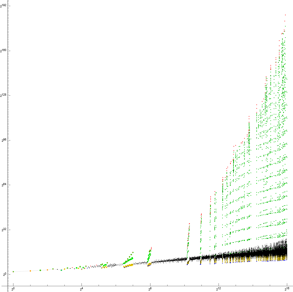
Figure T4: Log-log scatterplot of T(n), 13500 ≤ n ≤ 14500, expanding on powers pm conspicuously seen as echoes in larger plots, e.g., Figure T1.

Figure U3: Scatterplot of U(1…120), showing the even frontier (the zone defined by minima and maxima in the even terms), and the odd frontier (same pertaining to odd terms). This illustrates the prime divisor winnowing effect, which principally manifests a mild bifurcation of the sequence as to parity. Odd terms generally enter later than evens.

References:
[1] J. C. Lagarias, E. M. Rains, and N. J. A. Sloane, The EKG sequence, arXiv:math/0204011 [math.NT], 2002.
[2] Michael De Vlieger, Constitutive analysis of the EKG sequence, Sequence Analysis, 2021.
[3] Michael De Vlieger, Constitutive relations, Sequence Analysis, 2021.
[4] David L. Applegate, Hans Havermann, Bob Selcoe, Vladimir Shevelev, N. J. A. Sloane, and Reinhard Zumkeller, The Yellowstone Permutation, arXiv:1501.01669 [math.NT], 2015.
Code 1: Generate the constititive state between j and k:
conState[j_, k_] :=
Which[j == k, 5,
GCD[j, k] == 1, 0,
True, 1 + FromDigits[Map[Which[Mod[##] == 0, 1,
PowerMod[#1, #2, #2] == 0, 2, True, 0] & @@
# &, Permutations[{k, j}]], 3]]
Code S1: Generate S and store it in the variable a353916:
a353916 = Block[{nn = 120, a, c, k, s = {1, 2}, u = 1, state = {2, 3, 4, 7}},
c[_] = 0;
MapIndexed[Set[{a[First[#2]], c[#1]}, {#1, First[#2]}] &, s];
While[c[u] > 0, u++];
Monitor[Do[
Set[k, u];
While[Nand[c[k] == 0, MemberQ[state, conState[#, k]]], k++] &@ a[i - 1];
Set[{a[i], c[k]}, {k, i}];
If[k == u, While[c[u] > 0, u++]], {i, Length[s] + 1, nn}], i];
Array[a, nn]]
Code T1: Efficiently generate T using Theorem T5 and store it in the variable a353917:
a353917 = Block[{nn = 2^16 + 1, a, c, j, k, p, s = {4}, u = 3, state = {3, 7}},
c[_] = 0; p[_] = 2;
MapIndexed[Set[{a[First[#2]], c[#1]}, {#1, First[#2]}] &, s];
While[c[u] > 0, u++]; Set[j, s[[-1]]]; p[2] = 3;
Monitor[Do[
Set[k, u];
If[PrimeNu[j] == PrimeOmega[j] == 2,
k = Min[Map[#^p[#] &, FactorInteger[j][[All, 1]]]],
While[Nand[c[k] == 0, j != k, MemberQ[state, conState[j, k]]], k++]];
Set[{a[i], c[k]}, {k, i}];
j = k;
If[PrimePowerQ@ k, p[FactorInteger[k][[1, 1]]]++];
If[k == u, While[c[u] > 0, u++]], {i, Length[s] + 1, nn}], i];
Array[a, nn]]
Concerns sequences:
A006881: Squarefree semiprimes.
A007947: Squarefree kernel of n.
A064413: The EKG sequence.
A113552: EKG sequence restricted to asymmetric semicoprime divisorship states ②④.
A120944: Composite numbers m with ω(m) > 1 and are not squarefree, i.e., tantus numbers.
A126706:
Composite squarefree numbers, i.e., varius numbers.
A240024:
Seq. R. EKG sequence restricted to completely neutral constitutive states ①③⑦⑨.
A246547: Composite prime powers, i.e., multus numbers.
A336957: Enots Wolley sequence, a variation of Yellowstone intended to reverse axioms.
A337687: EKG sequence restricted to symmetric semicoprime constitutive state ①.
A350352: Products of 3 or more distinct prime numbers.
A353916: Sequence S. EKG sequence restricted to constitutive states ②③④⑦.
A353917: Sequence T. EKG sequence restricted to mixed neutral constitutive states ③⑦.
This work is dedicated to the memory of innocent children in Uvalde, Texas.
Document Revision Record.
2022 0517 2100 Draft 1.
2022 0525 2145 Draft 2.
2022 0526
1630 Add A240024 and A337687.
2022 0526 2145 Add A113552.
2022 0527 1045 Add A064413, outline, and summary of comparisons in conclusion.
2022 0531 1530 Final.
2022 0607 2230 Conjecture S7 added, prime divisor winnowing effect of A337687 illustrated.