Introduction Page 1

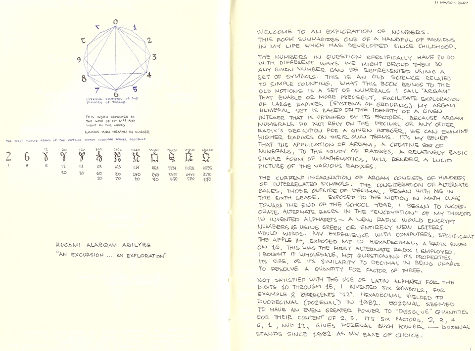
The introduction recounts the early development of argam and my childhood interest in number bases. This introduction developed after some of the sketchbook did, space reserved for an introduction, as it is a departure from pictorial work. The cyclic diagram for twelve appears, along with the argam for superior highly composite numbers. Cyclic diagrams were first sketched in 2006 on scratch paper, then made into digital studies. The diagrams were later hashed out in this book at s7836a06 and in the Rykami Arysane at s5231a90. This study developed into the 2009 Cyclic Resonance paper (800k PDF), and was incorporated into the March 2010 Balance Study (1¾ Mb PDF). Written 11 March 2007, tayya 790b (Salcyra Karlmelal, “Life Phase of Karl Michael, Son”), St. Louis.

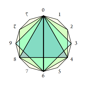
The “cyclical symmetry” graph at upper left was remastered 6 July 2018, Tayya a195, ten dozen first phase (Dejine-Anviantikymal Xrga, “life phase of Automated Charting”), St. Louis; it appears below.

cyclical symmetry graph of 12

Ultimate effect of the studies in this sketchbook

It is perhaps interesting to examine where the thoughts borne in the Rykami Argame sketchbook eventually led. This page mentions superior highly composite numbers.

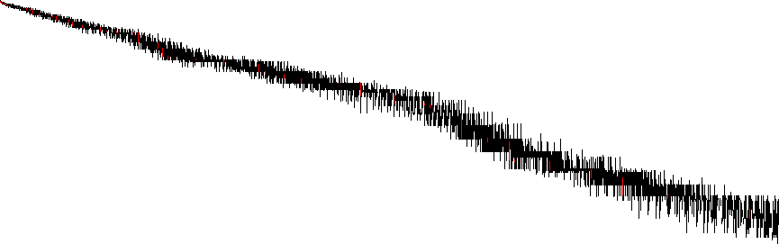
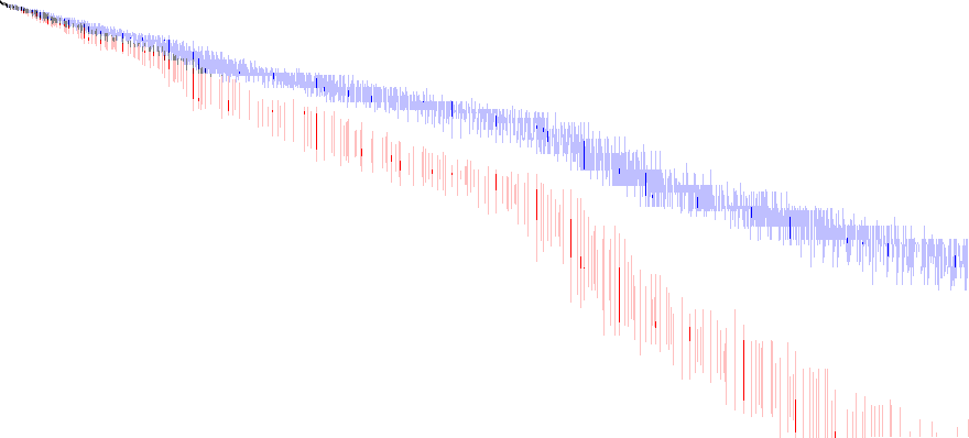
In spring 2018 (tayya a111), I was investigating the regular counting function of the highly composite divisors (i.e., A301892(n) = A010846(A002182(n))) and noted that the intersection of the HCNs and the highly regular numbers (i.e., A002182 and A244052) is finite at 13 terms (cf. A168263). I had plotted each HCN as an ordered pair, eventually leading to the processing of the 779674 terms Achim Flammenkamp described, and about which I had known at the time of drafting the Rykami Argame in 2008. In the chart below, we see highly composite m at (x, y) where the ordered pair represents the largest primorial that divides m, A002110(y) × A301414(x) = m. (The chart has y increasing downward, x increasing rightward). Superior highly composite numbers are plotted in red.

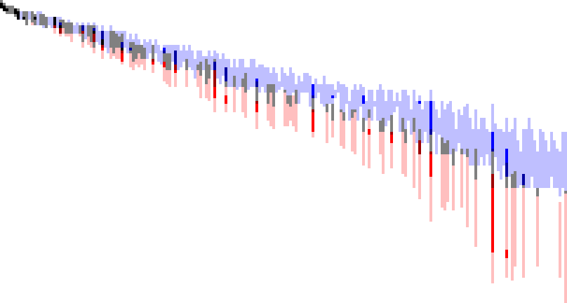
Later, this led to a chart shown below that derives from plotting highly composite (blue) or superabundant (red) m at (x, y) where the ordered pair represents the largest primorial that divides m, A002110(y) × A301414(x) = m. (The chart has y increasing downward, x increasing rightward). This resulted in posing several sequences in the OEIS (A301414, A304234, A304235) that derive from the chart below.

Writ large, this sort of plot illustrates the differences between the highly composite and superabundant numbers:

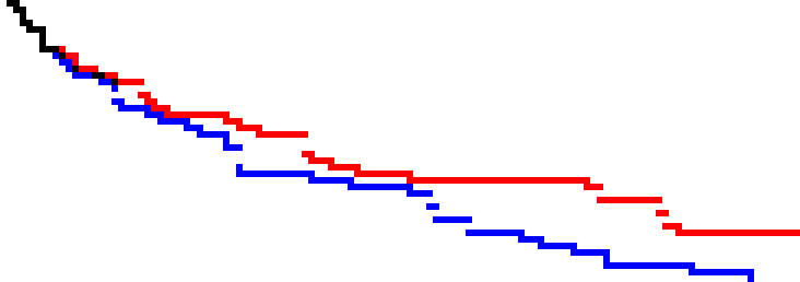
Plotting superior highly composite (red) and colossally abundant numbers (blue) results in the following graph, with the coordinates (x, y) flopped:

These charts were generated in Wolfram Mathematica 11.3 as a matter of course, as by mid 2018, I had mastered coding in Wolfram language, a language I had first acquired in January 2008. Read more about further examinations of the highly composite and superabundant numbers here.

This page last modified Tuesday 15 May 2018.